Chapter 9 Networks: The Basics

Jason Owen-Smith

Social scientists are typically interested in describing the activities of individuals and organizations (such as households and firms) in a variety of economic and social contexts. The frame within which data has been collected will typically have been generated from tax or other programmatic sources. The new types of data permit new units of analysis—particularly network analysis—largely enabled by advances in mathematical graph theory. This chapter provides an overview of how social scientists can use network theory to generate measurable representations of patterns of relationships connecting entities. The value of the new framework is not only in constructing different right-hand-side variables but also in studying an entirely new unit of analysis that lies somewhere between the largely atomistic actors that occupy the markets of neo-classical theory and the tightly managed hierarchies that are the traditional object of inquiry of sociologists and organizational theorists.

9.1 Introduction

Social Scientists have studied networks for a long time. A lot of the theory behind network analysis in fact comes from the social sciences where we studied relationships between people, groups, and organizations (Moreno 1934). What’s different today is the scale of the data available to us to perform this analysis. Instead of studying a group of 25 participants in a karate club (Zachary 1977), we now have data about hundreds of millions of people communicating with each other through social media channels, or hundreds of thousands of employees in a large multinational organizations collaborating on projects. This increased scale requires us to explore new methods of answering the same questions that we used to be interested in, as well as opens up avenues to answer new questions that could not be answered before.⁷³

Box: Network Analysis Examples

Example 1: Cascading Information⁷⁴ (Ugander et al. 2011). By using network analysis, researchers were able to characterize how information travels and recurs in patterns, exhibiting multiple bursts of popularity.
Example 2: Large-Scale Social Networks⁷⁵ (Stopczynski et al. 2014). Using data from a variety of sources to determine how people are connected, Stopczynski et al. are able to observe how communities form and social interactions change over time.
Example 3: Facebook Social Graph⁷⁶ (Cheng et al. 2016). A study of the Facebook friendship network was able to characterize how connected people were on the social networking site. By studying clustering and friendship preferences, the researchers were able to see how communities form and explore the “six degrees of separation” phenomenon on Facebook.

This chapter provides a basic introduction to the analysis of large networks for social science research and practice. We describe how to use data from existing social networks as well as how to turn “non-network” data into a network to perform further analysis. We then describe different measures that can be calculated to understand the properties of the network being analyzed, show different network visualization techniques, and discuss social science questions that these network measures and visualizations can help us answer.

We use the comparison of the collaboration networks of two research-intensive universities to show how to perform network analysis but the same approach generalizes to other types of problems. The collaboration networks and a grant co-employment network for a large public university examined in this chapter are derived from data produced by the multi-university Committee on Institutional Cooperation (CIC)’s UMETRICS project (Lane et al. 2015). The snippets of code that are provided are from the igraph package for network analysis as implemented in Python.

9.2 What are networks?

Networks are measurable representations of relationships connecting entities. What this means is that there are two fundamental questions to ask of any network representation: First, what are the nodes, or entities that are connected? Second, what are the relationships (ties or edges) connecting the nodes? Once we have the representation, we can then analyze the underlying data and relationships through the measures and methods described in this chapter. This is of great interest because a great deal of research in social sciences demonstrates that networks are essential to understanding behaviors and outcomes at both the individual and the organizational level.

Networks offer not just another convenient set of right-hand-side variables, but an entirely new unit of analysis that lies somewhere between the largely atomistic actors that occupy the markets of neo-classical theory and the tightly managed hierarchies that are the traditional object of inquiry of sociologists and organizational theorists. As Walter W. Powell (2003) puts it in a description of buyer supplier networks of small Italian firms: “when the entangling of obligation and reputation reaches a point where the actions of the parties are interdependent, but there is no common ownership or legal framework … such a transaction is neither a market exchange nor a hierarchical governance structure, but a separate, different mode of exchange.”

Existing as they do between the uncoordinated actions of independent individuals and coordinated work of organizations, networks offer a unique level of analysis for the study of scientific and creative teams (Wuchty, Jones, and Uzzi 2007), collaborations (Kabo et al. 2015), and clusters of entrepreneurial firms (Owen-Smith and Powell 2004).

The following sections will introduce you to this approach to studying innovation and discovery, focusing on examples drawn from high-technology industries and particularly from the scientific collaborations among grant-employed researchers at UMETRICS universities. We make particular use of a network that connects individual researchers to grants that paid their salaries in 2012 for a large public university. The grants network for university A includes information on 9,206 individuals who were employed on 3,389 research grants from federal science agencies in a single year. The web of partnerships that emerges from university scientists’ decentralized efforts to build effective collaborations and teams generates a distinctive social infrastructure for cutting-edge science.

While this chapter focuses on social networks, the techniques described here have been used to examine the structure of networks such as the World Wide Web, the national railway route map of the USA, the food web of an ecosystem, or the neuronal network of a particular species of animal.

9.3 Structure for this chapter

The chapter first introduces the most common structures for large network data, briefly introduce three key social “mechanisms of action” by which social networks are thought to have their effects, and then present a series of basic measures that can be used to quantify characteristics of entire networks and the relative position individual people or organizations hold in the differentiated social structure created by networks.

Taken together, these measures offer an excellent starting point for examining how global network structures create opportunities and challenges for the people in them, for comparing and explaining the productivity of collaborations and teams, and for making sense of the differences between organizations, industries, and markets that hinge on the pattern of relationships connecting their participants.

Understanding the productivity and effects of university research thus requires an effort to measure and characterize the networks on which it depends. As suggested, those networks influence outcomes in three ways: first, they distinguish among individuals; second, they differentiate among teams; and third, they help to distinguish among research-performing universities. Most research-intensive institutions have departments and programs that cover similar arrays of topics and areas of study. What distinguishes them from one another is not the topics they cover but the ways in which their distinctive collaboration networks lead them to have quite different scientific capabilities.

9.4 Turning Data into a Network

Networks are comprised of nodes, which represent entities that can be connected to one another, and of ties that represent the relationships connecting nodes. When ties are undirected (representing a relationship between the nodes that is not directional) they are called edges. When they are directed (as when I lend money to you and you do or do not reciprocate) they are called arcs. Nodes, edges and arcs can, in principle, be anything: patents and citations, web pages and hypertext links, scientists and collaborations, teenagers and intimate relationships, nations and international trade agreements. The very flexibility of network approaches means that the first step toward doing a network analysis is to first turn our data into a graph by clearly defining what counts as a node and what counts as a tie. In traditional social network analysis studies, there is a natural representation of the data as a network. People are often nodes, and some type of communication between them form the “ties”. While this seems like an easy move, it often requires deep thought. For instance, an interest in innovation and discovery could take several forms. We could be interested in how universities differ in their capacity to respond to new requests for proposals (a macro question that would require the comparison of full networks across campuses). We could wonder what sorts of training arrangements lead to the best outcomes for graduate students (a more micro-level question that requires us to identify individual positions in larger networks). Or we could ask what team structure is likely to lead to more or less radical discoveries (a decidedly meso-level question that requires we identify substructures and measure their features).

Each of these is a network question that relies on the ways in which people are connected to one another. The first challenge of measurement is to identify the nodes (what is being connected) and the ties (the relationships that matter) in order to construct the relevant networks. The next is to collect and structure the data in a fashion that is sufficient for analysis. Finally, measurement and visualization decisions must be made.

9.4.1 Types of Networks

Network ties can be directed (flowing from one node to another) or undirected. In either case they can be binary (indicating the presence or absence of a tie) or valued (allowing for relationships of different types or strengths). Network data can be represented in matrices or as lists of edges and arcs. All these types of relationships can connect one type of node (what is commonly called one-mode network data) or multiple types of nodes (what is called two-mode or affiliation data). Varied data structures correspond to different classes of network data. The simplest form of network data represents instances where the same kinds of nodes are connected by undirected ties (edges) that are binary. An example of this type of data is a network where nodes are firms and ties indicate the presence of a strategic alliance connecting them (Powell et al. 2005). This network would be represented as a square symmetric matrix or a list of edges connecting nodes. Figure 9.1 summarizes this simple data structure, highlighting the idea that network data of this form can be represented either as a matrix or as an edge list. If this data was representing acquisitions, we could turn it into a directed graph where the edge would be directed from the acquiring firm to the acquired firm.

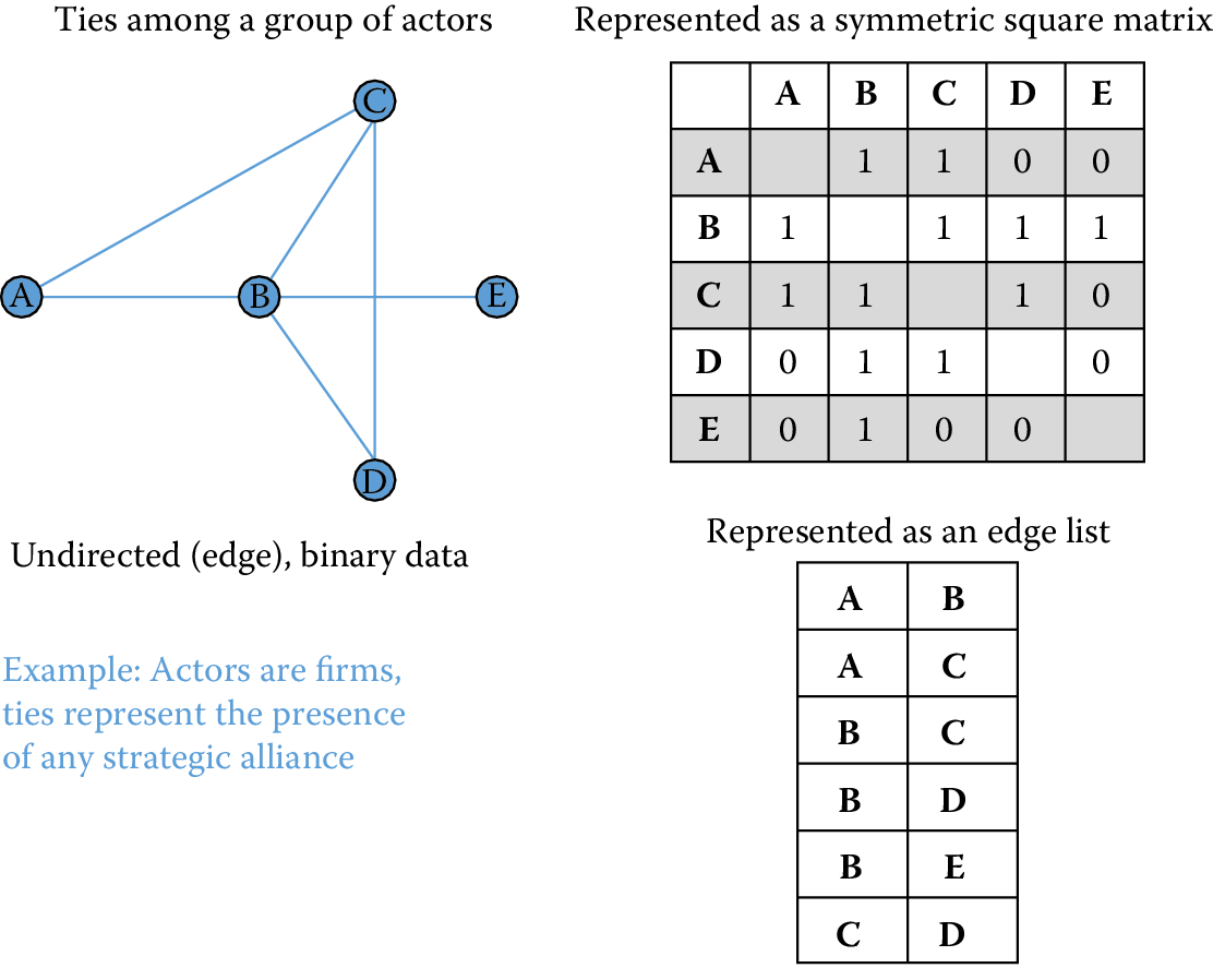
Figure 9.1: Undirected, binary, one-mode network data

A much more complicated network would be one that is both directed and valued. One example might be a network of nations connected by flows of international trade. Goods and services flow from one nation to another and the value of those goods and services (or their volume) represents ties of different strengths. When networks connecting one class of nodes (in this case nations) are directed and valued, they can be represented as asymmetric valued matrices or lists of arcs with associated values. (See Figure 9.1.)

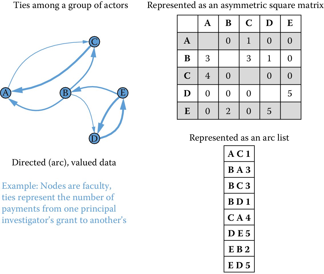
Figure 9.2: Directed, valued, one-mode network data

Many studies of small- to medium-sized social networks rely on one-mode data. Large-scale social network data of this type are relatively rare, but one-mode data of this sort are fairly common in relationships among other types of nodes such as web pages or citations connecting patents or publications. Nevertheless, much “big” social network analysis is conducted using two-mode data. The UMETRICS employee data set is a two-mode network that connects people (research employees) to the grants that pay their wages. These two types of nodes can be represented as a rectangular matrix that is either valued or binary. It is relatively rare to analyze untransformed two-mode network data. Instead, most analyses take advantage of the fact that such networks are dual (White, Boorman, and Breiger 1976). In other words, a two-mode network connecting grants and people can be conceptualized (and analyzed) as two one-mode networks, or projections⁷⁷.

9.4.2 Inducing one-mode networks from two-mode data

The most important trick in large-scale social network analysis is that of inducing one-mode, or unipartite, networks (e.g., employee $\times$ employee relationships) from two-mode, or bipartite, data. But the ubiquity and potential value of two-mode data can come at a cost. Not all affiliations are equally likely to represent real, meaningful relationships. While it seems plausible to assume that two individuals paid by the same grant have interactions that reasonably pertain to the work funded by the grant, this need not be the case.

For example, consider the two-mode grant $\times$ person network for university A. I used SQL to create a representation of this network that is readable by a freeware network visualization program called Pajek (Batagelj and Mrvar 1998). In this format, a network is represented as two lists: a vertex list that lists the nodes in the graph and an edge list that lists the connections between those nodes. In our grant $\times$ person network, we have two types of nodes, people and grants, and one kind of edge, used to represent wage payments from grants to individuals.

I present a brief snippet of the resulting network file in what follows, showing first the initial 10 elements of the vertex list and then the initial 10 elements of the edge list, presented in two columns for compactness. (The complete file comprises information on 9,206 employees and 3,389 grants, for a total of 12,595 vertices and 15,255 edges. The employees come first in the vertex list, and so the 10 rows shown below all represent employees.) Each vertex is represented by a vertex number–label pair and each edge by a pair of vertices plus an optional value. Thus, the first entry in the edge list (1 10419) specifies that the vertex with identifier 1 (which happens to be the first element of the vertex list, which has value “00100679”) is connected to the vertex with identifier 10419 by an edge with value 1, indicating that employee “00100679” is paid by the grant described by vertex 10419.

*Grant-Person-Network

*Vertices 12595 9206		*Edges
1	“00100679”	1	10419
2	“00107462”	2	10422
3	“00109569”	3	9855
4	“00145355”	3	9873
5	“00153190”	4	9891
6	“00163131”	7	10432
7	“00170348”	7	12226
8	“00172339”	8	10419
9	“00176582”	9	11574
10	“00203529”	10	11196

The network excerpted above is two-mode because it represents relationships between two different classes of nodes, grants, and people. In order to use data of this form to address questions about patterns of collaboration on UMETRICS campuses, we must first transform it to represent collaborative relationships.

A person-by-person projection of the original two-mode network assumes that ties exist between people when they are paid by the same grant. By the same token, a grant-by-grant projection of the original two-mode network assumes that ties exist between grants when they pay the same people. Transforming two-mode data into one-mode projections is a fairly simple matter. If $\mathbf{X}$ is a rectangular matrix, $p \times g$, then a one-mode projection, $p \times p$, can be obtained by multiplying $\mathbf{X}$ by its transpose $\mathbf{X}'$. Figure 9.3 summarizes this transformation.

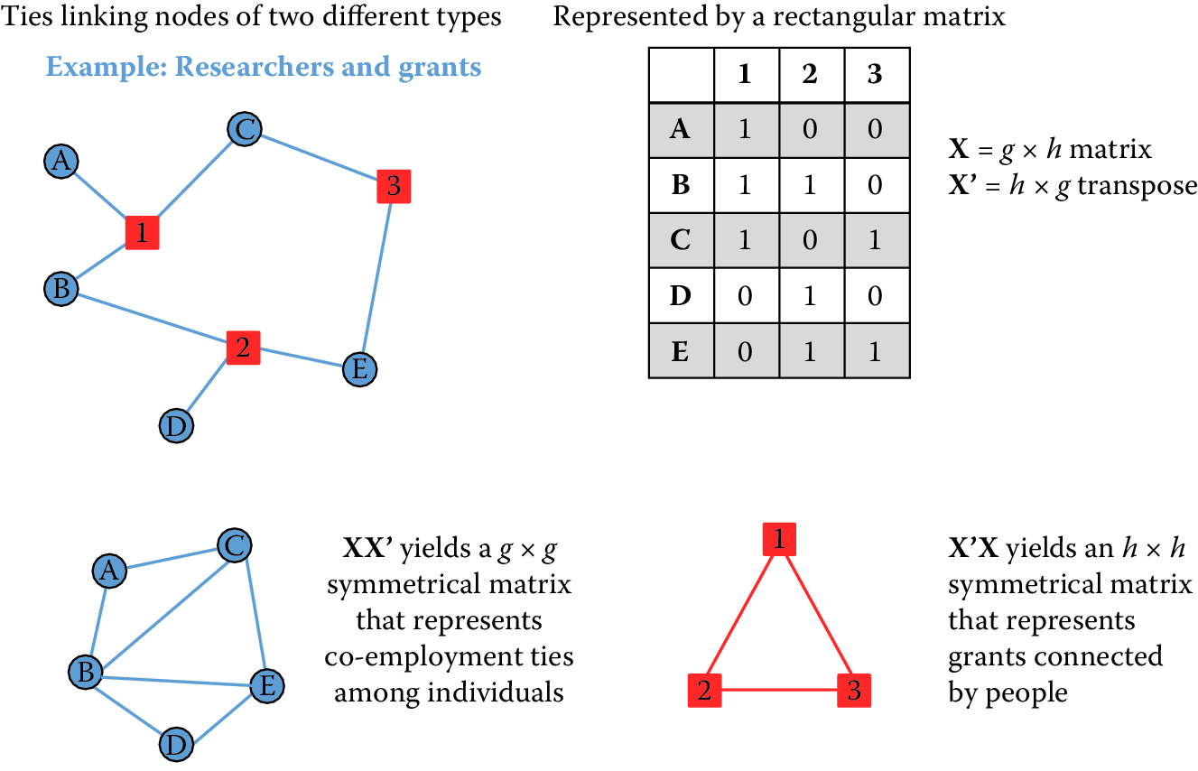
Figure 9.3: Two-mode affiliation data

In the following snippet of code, I use the igraph package in Python to read in a Pajek file and then transform the original two-mode network into two separate projections. Because my focus in this discussion is on relationships among people, I then move on to work exclusively with the employee-by-employee projection. However, every technique that I describe below can also be used with the grant-by-grant projection, which provides a different view of how federally funded research is put together by collaborative relationships on campus.

from igraph import *

# Read the graph
g = Graph.Read_Pajek("public_a_2m.net")

# Look at result
summary(g)


# IGRAPH U-WT 12595 15252 --
# + attr: color (v), id (v), shape (v), type (v), x (v), y (v), z (v), weight (e)
# ...
# ...

# Transform to get 1M projection
pr_g_proj1, pr_g_proj2= g.bipartite_projection()

# Look at results
summary(pr_g_proj1)

# IGRAPH U-WT 9206 65040 --
# + attr: color (v), id (v), shape (v), type (v), x (v), y (v), z (v), weight (e)

summary(pr_g_proj2)
# IGRAPH U-WT 3389 12510 --
# + attr: color (v), id (v), shape (v), type (v), x (v), y (v), z (v), weight (e)

# pr_g_proj1 is the employeeXemployee projection, n=9,206 nodes
# Rename to emp for use in future calculations

emp=pr_g_proj1

We now can work with the graph emp, which represents the collaborative network of federally funded research on this campus. Care must be taken when inducing one-mode network projections from two-mode network data because not all affiliations provide equally compelling evidence of actual social relationships. While assuming that people who are paid by the same research grants are collaborating on the same project seems plausible, it might be less realistic to assume that all students who take the same university classes have meaningful relationships. For the remainder of this chapter, the examples I discuss are based on UMETRICS employee data rendered as a one-mode person-by-person projection of the original two-mode person-by-grants data. In constructing these networks I assume that a tie exists between two university research employees when they are paid any wages from the same grant during the same year. Other time frames or thresholds might be used to define ties if appropriate for particular analyses⁷⁸.

9.5 Network measures

The power of networks lies in their unique flexibility and ability to address many phenomena at multiple levels of analysis. But harnessing that power requires calculating measures that take into account the overall structure of relationships represented in a given network. The key insight of structural analysis is that outcomes for any individual or group are a function of the complete pattern of connections among them. In other words, the explanatory power of networks is driven as much by the pathways that indirectly connect nodes as by the particular relationships that directly link members of a given dyad. Indirect ties create reachability in a network⁷⁹.

9.5.1 Reachability

Two nodes are said to be reachable when they are connected by an unbroken chain of relationships through other nodes. For instance, two people who have never met may nonetheless be able to reach each other through a common acquaintance who is positioned to broker an introduction (Obstfeld 2005) or the transfer of information and resources (Burt 2004). It is the reachability that networks create that makes them so important for understanding the work of science and innovation.

Consider Figure 9.4, which presents three schematic networks. In each, one focal node, ego, is colored orange. Each ego has four alters, but the fact that each has connections to four other nodes masks important differences in their structural positions. Those differences have to do with the number of other nodes they can reach through the network and the extent to which the other nodes in the network are connected to each other. The orange node (ego) in each network has four partners, but their positions are far from equivalent. Centrality measures on full network data can tease out the differences. The networks also vary in their gross characteristics. Those differences, too, are measurable⁸⁰.

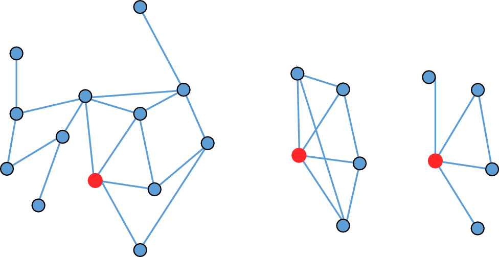
Figure 9.4: Reachability and indirect ties

Networks in which more of the possible connections among nodes are realized are denser and more cohesive than networks in which fewer potential connections are realized. Consider the two smaller networks in Figure 9.4, each of which is comprised of five nodes. Just five ties connect those nodes in the network on the far right of the figure. One smaller subset of that network, the triangle connecting ego and two alters at the center of the image, represents a more cohesively connected subset of the networks. In contrast, eight of the nine ties that are possible connect the five nodes in the middle figure; no subset of those nodes is clearly more interconnected than any other. While these kinds of differences may seem trivial, they have implications for the orange nodes, and for the functioning of the networks as a whole. Structural differences between the positions of nodes, the presence and characteristics of cohesive “communities” within larger networks (Girvan and Newman 2002), and many important properties of entire structures can be quantified using different classes of network measures. Newman (2010) provides the most recent and most comprehensive look at measures and algorithms for network research.

The most essential thing to be able to understand about larger scale networks is the pattern of indirect connections among nodes. What is most important about the structure of networks is not necessarily the ties that link particular pairs of nodes to one another. Instead, it is the chains of indirect connections that make networks function as a system and thus make them worthwhile as new levels of analysis for understanding social and other dynamics.

9.5.2 Whole-network measures

The basic terms needed to characterize whole networks are fairly simple. It is useful to know the size (in terms of nodes and ties) of each network you study. This is true both for the purposes of being able to generally gauge the size and connectivity of an entire network and because many of the measures that one might calculate using such networks should be standardized for analytic use. While the list of possible network measures is long, a few commonly used indices offer useful insights into the structure and implications of entire network structures.

Components and reachability

As we have seen, a key feature of networks is reachability. The reachability of participants in a network is determined by their membership in what network theorists call components, subsets of larger networks where every member of a group is indirectly connected to every other. If you imagine a standard node and line drawing of a network, a component is a portion of the network where you can trace paths between every pair of nodes without ever having to lift your pen.

Most large networks have a single dominant component that typically includes anywhere from 50% to 90% of its participants as well as many smaller components and isolated nodes that are disconnected from the larger portion of the network. Because the path length centrality measures described below can only be computed on connected subsets of networks, it is typical to analyze the largest component of any given network. Thus any description of a network or any effort to compare networks should report the number of components and the percentage of nodes reachable through the largest component. In the code snippet below, I identify the weakly connected components of the employee network, emp.

# Add component membership
emp.vs["membership"] = emp.clusters(mode="weak").membership

# Add component size
emp.vs["csize"] = [emp.clusters(mode="weak").sizes()[i] for i in emp.clusters(mode="weak").membership]

# Identify the main component
# Get indices of max clusters
maxSize = max(emp.clusters(mode="weak").sizes())
emp.vs["largestcomp"] = [1 if maxSize == x else 0 for x in emp.vs["csize"]]

# Add component membership

emp.vs["membership"] = emp.clusters(mode="weak").membership

The main component of a network is commonly analyzed and visualized because the graph-theoretic distance among unconnected nodes is infinite, which renders calculation of many common network measures impossible without strong assumptions about just how far apart unconnected nodes actually are. While some researchers replace infinite path lengths with a value that is one plus the longest path, called the network’s diameter, observed in a given structure, it is also common to simply analyze the largest connected component of the network.

Path length

One of the most robust and reliable descriptive statistics about an entire network is the average path length, $l_{G}$, among nodes. Networks with shorter average path lengths have structures that may make it easier for information or resources to flow among members in the network. Longer path lengths, by comparison, are associated with greater difficulty in the diffusion and transmission of information or resources. Let $g$ be the number of nodes or vertices in a network. Then \[l_G=\frac{1}{g(g-1)}\sum_{i\neq j}d(n_i,n_j),\] where $d(n_i,n_j)$ is the path length between $n_i$ and $n_j$. Typically, the path length is defined as the length of the shortest path⁸¹ between two nodes.

As with other measures based on reachability, it is most common to report the average path length for the largest connected component of the network because the graph-theoretic distance between two unconnected nodes is infinite. In an electronic network such as the World Wide Web, a shorter path length means that any two pages can be reached through fewer hyperlink clicks.

The snippet of code below identifies the distribution of shortest path lengths among all pairs of nodes in a network and the average path length. I also include a line of code that calculates the network distance among all nodes and returns a matrix of those distances. That matrix (saved as empdist) can be used to calculate additional measures or to visualize the graph-theoretic proximities among nodes.

# Calculate distances and construct distance table

dfreq=emp.path_length_hist(directed=False)
print(dfreq)

# N = 12506433, mean +- sd: 5.0302 +- 1.7830
# Each * represents 51657 items
# [ 1,  2): * (65040)
# [ 2,  3): ********* (487402)
# [ 3,  4): *********************************** (1831349)
# [ 4,  5): ********************************************************** (2996157)
# [ 5,  6): **************************************************** (2733204)
# [ 6,  7): ************************************** (1984295)
# [ 7,  8): ************************ (1267465)
# [ 8,  9): ************ (649638)
# [ 9, 10): ***** (286475)
# [10, 11): ** (125695)
# [11, 12): * (52702)
# [12, 13):  (18821)
# [13, 14):  (5944)
# [14, 15):  (1682)
# [15, 16):  (403)
# [16, 17):  (128)
# [17, 18):  (28)
# [18, 19):  (5)
print(dfreq.unconnected)
# 29864182

print(emp.average_path_length(directed=False))
#[1] 5.030207

empdist= emp.shortest_paths()

These measures provide a few key insights into the employee network we have been considering. First, the average pair of nodes that are connected by indirect paths are slightly more than five steps from one another. Second, however, many node pairs in this network ($unconnected = 29,864,182) are unconnected and thus unreachable to each other. Figure 9.5 presents a histogram of the distribution of path lengths in the network. It represents the numeric values returned by the distance.table command in the code snippet above. In this case the diameter of the network is 18 and five pairs of nodes are reachable at this distance, but the largest group of dyads is reachable ($N=2{,}996{,}157$ dyads) at distance 4. In short, nearly 3 million pairs of nodes are collaborators of collaborators of collaborators of collaborators.

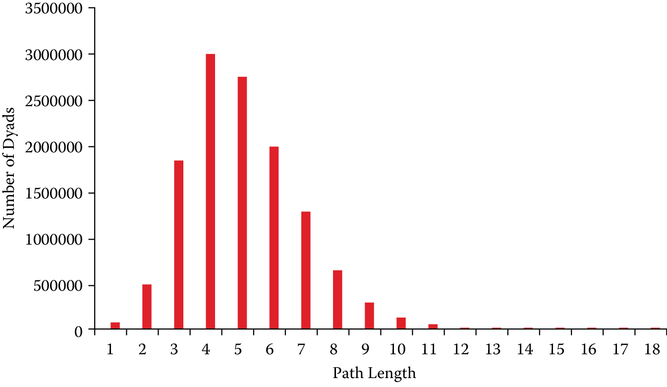
Figure 9.5: Histogram of path lengths for university A employee network

Degree distribution

Another powerful way to describe and compare networks is to look at the distribution of centralities across nodes. While any of the centrality measures described above could be summarized in terms of their distribution, it is most common to plot the degree distribution of large networks. Degree distributions commonly have extremely long tails. The implication of this pattern is that most nodes have a small number of ties (typically one or two) and that a small percentage of nodes account for the lion’s share of a network’s connectivity and reachability. Degree distributions are typically so skewed that it is common practice to plot degree against the percentage of nodes with that degree score on a log–log scale.

High-degree nodes are often particularly important actors. In the UMETRICS networks that are employee $\times$ employee projections of employee $\times$ grant networks, for instance, the nodes with the highest degree seem likely to include high-profile faculty—the investigators on larger institutional grants such as National Institutes of Health-funded Clinical and Translational Science Awards and National Science Foundation-funded Science and Technology Centers, and perhaps staff whose particular skills are in demand (and paid for) by multiple research teams. For instance, the head technician in a core microscopy facility or a laboratory manager who serves multiple groups might appear highly central in the degree distribution of a UMETRICS network.

Most importantly, the degree distribution is commonly taken to provide insight into the dynamics by which a network was created. Highly skewed degree distributions often represent scale-free networks (Powell et al. 2005; Barabási and Albert 1999; Newman 2005), which grow in part through a process called preferential attachment, where new nodes entering the network are more likely to attach to already prominent participants. In the kinds of scientific collaboration networks that UMETRICS represents, a scale-free degree distribution might come about as faculty new to an institution attempt to enroll more established colleagues on grants as coinvestigators. In the comparison exercise outlined below, I plot degree distributions for the main components of two different university networks.

Clustering coefficient

The third commonly used whole-network measure captures the extent to which a network is cohesive, with many nodes interconnected. In networks that are more cohesively clustered, there are fewer opportunities for individuals to play the kinds of brokering roles that we will discuss below in the context of betweenness centrality. Less cohesive networks, with lower levels of clustering, are potentially more conducive to brokerage and the kinds of innovation that accompany it.

However, the challenge of innovation and discovery is both the moment of invention, the “aha!” of a good new idea, and the often complicated, uncertain, and collaborative work that is required to turn an initial insight into a scientific finding. While less clustered, open networks are more likely to create opportunities for brokers to develop fresh ideas, more cohesive and clustered networks support the kinds of repeated interactions, trust, and integration that are necessary to do uncertain and difficult collaborative work.

While it is possible to generate a global measure of cohesiveness in networks, which is generically the number of closed triangles (groups of three nodes all connected to one another) as a proportion of the number of possible triads, it is more common to take a local measure of connectivity and average it across all nodes in a network. This local connectivity measure more closely approximates the notion of cohesion around nodes that is at the heart of studies of networks as means to coordinate difficult, risky work. The code snippet below calculates both the global clustering coefficient and a vector of node-specific clustering coefficients whose average represents the local measure for the employee $\times$ employee network projection of the university A UMETRICS data.

# Calculate clustering coefficients
emp.transitivity_undirected()
# 0.7241

local_clust=emp.transitivity_local_undirected(mode="zero")
# (isolates="zero" sets clustering to zero rather than undefined)

import pandas as pd
print(pd.Series(local_clust).describe())
# count    9206.000000
# mean        0.625161
# std         0.429687
# min         0.000000
# 25%         0.000000
# 50%         0.857143
# 75%         1.000000
# max         1.000000
#--------------------------------------------------#

Together, these summary statistics—number of nodes, average path length, distribution of path lengths, degree distribution, and the clustering coefficient—offer a robust set of measures to examine and compare whole networks. It is also possible to distinguish among the positions nodes hold in a particular network. Some of the most powerful centrality measures also rely on the idea of indirect ties⁸².

Centrality measures

This class of measures is the most common way to distinguish between the positions individual nodes hold in networks. There are many different measures of centrality that capture different aspects of network positions, but they fall into three general types. The most basic and intuitive measure of centrality, degree centrality, simply counts the number of ties that a node has. In a binary undirected network, this measure resolves into the number of unique alters each node is connected to. In mathematical terms it is the row or column sum of the adjacency matrix that characterizes a network. Degree centrality, $C_{D}(n_{i})$, represents a clear measure of the prominence or visibility of a node. Let \[C_D(n_i)=\sum_jx_{ij}.\] The degree of a node is limited by the size of the network in which it is embedded. In a network of $g$ nodes the maximum degree of any node is $g-1$. The two orange nodes in the small networks presented in Figure 9.4 have the maximum degree possible (4). In contrast, the orange node in the larger, 13-node network in that figure has the same number of alters but the possible number of partners is three times as large (12). For this reason it is problematic to compare raw degree centrality measures across networks of different sizes. Thus, it is common to normalize degree by the maximum value defined by $g-1$: \[C_D^{\prime}(n_i)=\frac{\sum_j x_{ij}}{g-1}.\]

While the normalized degree centrality of the two orange nodes of the smaller networks in Figure 9.4 is 1.0, the normalized value for the node in the large network of 13 nodes is 0.33. Despite the fact that the highlighted nodes in the two smaller networks have the same degree centrality, the pattern of indirect ties connecting their alters means they occupy meaningfully different positions. There are a number of degree-based centrality measures that take more of the structural information from a complete network into account by using a variety of methods to account not just for the number of partners a particular ego might have but also for the prominence of those partners. Two well-known examples are eigenvector centrality and page rank (see Newman (2010) Ch. 7.2 and 8.4).

Consider two additional measures that capture aspects of centrality that have more to do with the indirect ties that increase reachability. Both make explicit use of the idea that reachability is the source of many of the important social and economic benefits of salutary network positions, but they do so with different substantive emphases. Both of these approaches rely on the idea of a network geodesic, the shortest path connecting any pair of actors. Because these measures rely on reachability, they are only useful when applied to components. When nodes have no ties (degree 0) they are called isolates. The geodesic distances are infinite and thus path-based centrality measures cannot be calculated. This is a shortcoming of these measures, which can only be used on connected subsets of graphs where each node has at least one tie to another and all are indirectly connected.

Closeness centrality, $C_{C,}$ is based on the idea that networks position some individuals closer to or farther away from other participants. The primary idea is that shorter network paths between actors increase the likelihood of communication and with it the ability to coordinate complicated activities. Let $d(n_{i}, n_{j})$ represent the number of network steps in the geodesic path connecting two nodes $i$ and $j$. As $d$ increases, the network distance between a pair of nodes grows. Thus a standard measure of closeness is the inverse of the sum of distances between any given node and all the others that are reachable in a network: \[C_C(n_i) = \frac{1}{\sum_{j=1}^gd(n_i,n_j)}.\] The maximum of closeness centrality occurs when a node is directly connected to every possible partner in the network. As with degree centrality, closeness depends on the number of nodes in a network. Thus, it is necessary to standardize the measure to allow comparisons across multiple networks: \[C_C^{\prime}(n_i)=\frac{g-1}{\sum_{j=1}^gd(n_i,n_j)}.\]

Like closeness centrality, betweenness centrality, $C_{B}$, relies on the concept of geodesic paths to capture nuanced differences the positions of nodes in a connected network. Where closeness assumes that communication and the flow of information increase with proximity, betweenness captures the idea of brokerage that was made famous by Burt (1993). Here too the idea is that flows of information and resources pass between nodes that are not directly connected through indirect paths. The key to the idea of brokerage is that such paths pass through nodes that can interdict, or otherwise profit from their position “in between” unconnected alters. This idea has been particularly important in network studies of innovation (Owen-Smith and Powell 2003; Burt 2004), where flows of information through strategic alliances among firms or social networks connecting individuals loom large in explanations of why some organizations or individuals are better able to develop creative ideas than others.

To calculate betweenness as originally specified, two strong assumptions are required (Freeman 1979). First, one must assume that when people (or organizations) search for new information through their networks, they are capable of identifying the shortest path to what they seek. When multiple paths of equal length exist, we assume that each path is equally likely to be used. Newman (2005) describes an alternative betweenness measure based on random paths through a network, rather than shortest paths, that relaxes these assumptions. For now, let $g_{jk}$ equal the number of geodesic paths linking any two actors. Then $1/g_{jk}$ is the probability that any given path will be followed on a particular node’s search for information or resources in a network. In order to calculate the betweenness score of a particular actor, $i$, it is then necessary to determine how many of the geodesic paths connecting $j$ to $k$ include $i$. That quantity is $g_{jk}(n_{i})$. With these (unrealistic) assumptions in place, we calculate $C_{B}(n_{i})$ as \[C_B(n_i)=\sum_{j<k} g_{jk}^{(n_i)}/g_{jk}.\] Here, too, the maximum value depends on the size of the network. $C_{B}(n_{i}) = 1$ if $i$ sits on every geodesic path in the network. While this is only likely to occur in small, star-shaped networks, it is still common to standardize the measure. Instead of conceptualizing network size in terms of the number of nodes, however, this measure requires that we consider the number of possible pairs of actors (excluding ego) in a structure. When there are $g$ nodes, that quantity is $(g-1)(g-2)/2$ and the standardized betweenness measure is \[C_B^{\prime}(n_i)=\frac{C_B(n_i)}{(g-1)(g-2)/2}.\]

Centrality measures of various sorts are the most commonly used means to examine network effects at the level of individual participants in a network. In the context of UMETRICS, such indices might be applied to examine the differential scientific or career success of graduate students as a function of their positions in the larger networks of their universities. In such an analysis, care must be taken to use the standardized measures as university collaboration networks can vary dramatically in size and structure. Describing and accounting for such variations and the possibility of analyses conducted at the level of entire networks or subsets of networks, such as teams and labs, requires a different set of measures. The code snippet presented below calculates each of these measures for the university A employee network we have been examining.

# Calculate centrality measures
emp.vs["degree"]=emp.degree()
emp.vs["close"]=emp.closeness(vertices=emp.vs)
emp.vs["btc"]=emp.betweenness(vertices=emp.vs, directed=False)

9.6 Case Study: Comparing collaboration networks

Consider Figure 9.6, which presents visualizations of the main component of two university networks. Both of these representations are drawn from a single year (2012) of UMETRICS data. Nodes represent people, and ties reflect the fact that those individuals were paid with the same federal grant in the same year. The images are scaled so that the physical location of any node is a function of its position in the overall pattern of relationships in the network. The size and color of nodes represent their betweenness centrality. Larger, darker nodes are better positioned to play the role of brokers in the network. A complete review of the many approaches to network visualization and their dangers in the absence of descriptive statistics such as those presented above is beyond the scope of this chapter, but consider the guidelines presented in Chapter Information Visualization on information visualization as well as useful discussions by Powell et al. (2005) and Healy and Moody (2014).

Consider the two images. University A is a major public institution with a significant medical school. University B, likewise, is a public institution but lacks a medical school. It is primarily known for strong engineering. The two networks manifest some interesting and suggestive differences. Note first that the network on the left (university A) appears much more tightly connected. There is a dense center and there are fewer very large nodes whose positions bridge less well-connected clusters. Likewise, the network on the right (university B) seems at a glance to be characterized by a number of densely interconnected groups that are pulled together by ties through high-degree brokers. One part of this may have to do with the size and structure of university A’s medical school, whose significant NIH funding dominates the network. In contrast, university B’s engineering-dominated research portfolio seems to be arranged around clusters of researchers working on similar topic areas and lacks the dominant central core apparent in university B’s image.

The implications of these kinds of university-level differences are just starting to be realized, and the UMETRICS data offer great possibilities for exactly this kind of study. These networks, in essence, represent the local social capacity to respond to new problems and to develop scientific findings. Two otherwise similar institutions might have quite different capabilities based on the structure and composition of their collaboration networks.

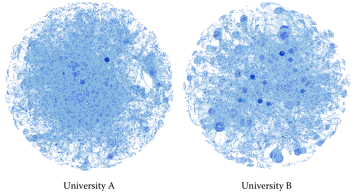
Figure 9.6: The main component of two university networks

The intuitions suggested by Figure 9.6 can also be checked against some of the measures we have described. Figure 9.7, for instance, presents degree distributions for each of the two networks. Figure 9.8 presents the histogram of path lengths for each network.

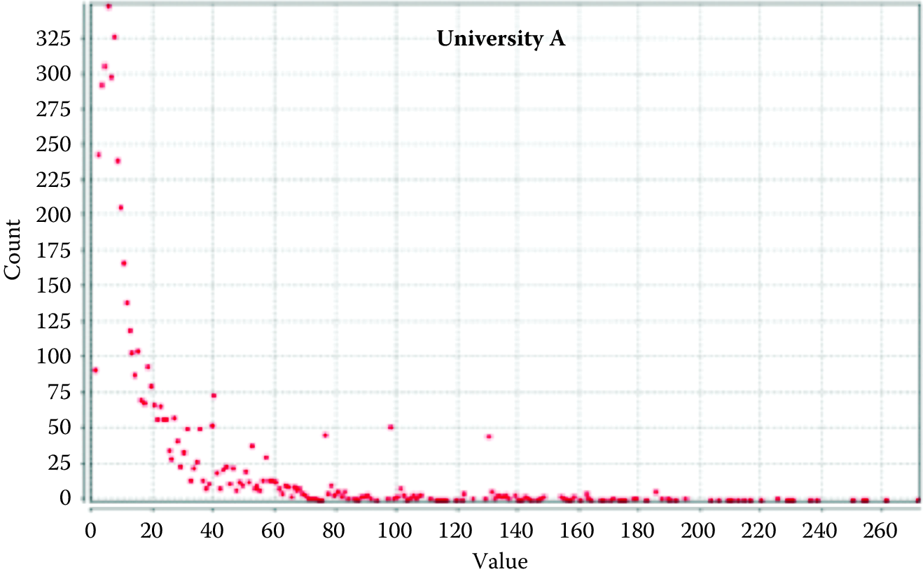
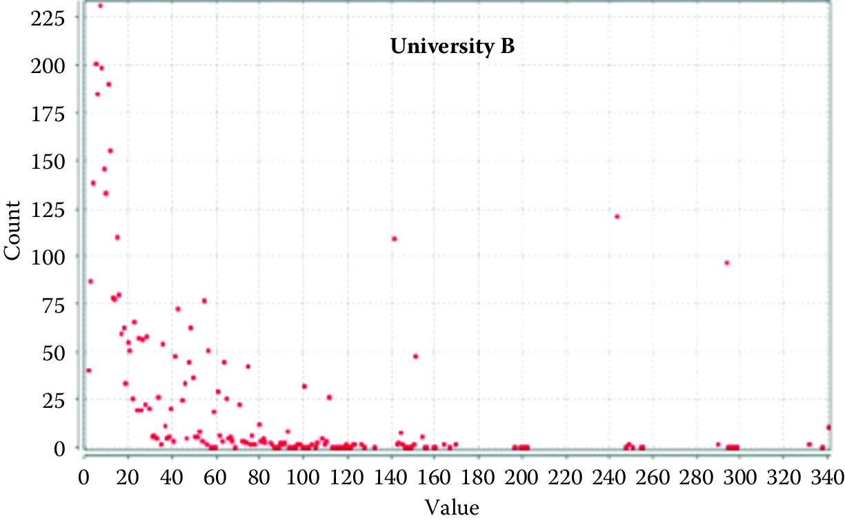
Figure 9.7: Degree distribution for two universities

It is evident from Figure 9.7 that they are quite different in character. University A’s network follows a more classic skewed distribution of the sort that is often associated with the kinds of power-law degree distributions common to scale-free networks. In contrast, university B’s distribution has some interesting features. First, the left-hand side of the distribution is more dispersed than it is for university A, suggesting that there are many nodes with moderate degree. These nodes may also have high betweenness centrality if their ties allow them to span different subgroups within the networks. Of course this might also reflect the fact that each cluster also has members that are more locally prominent. Finally, consider the few instances on the right-hand end of the distribution where there are relatively large numbers of people with surprisingly high degree. I suspect these are the result of large training grants or center grants that employ many people. A quirk of relying on one-mode projections of two-mode data is that every person associated with a particular grant is connected to every other. More work needs to be done to bear out these hypotheses, but for now it suffices to say that the degree distribution of the networks bears out the intuition we drew from the images that they are significantly different.

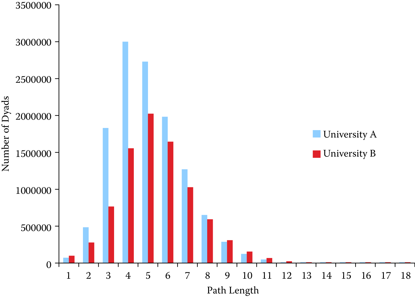
Figure 9.8: Distribution of path lengths for universities A and B

The path length histogram presented in Figure 9.8 suggests a similar pattern. While the average distance among any pair of connected nodes in both networks is fairly similar (see Table 9.1, university B has a larger number of unconnected nodes and university A has a greater concentration of more closely connected dyads. The preponderance of shorter paths in this network could also be a result of a few larger grants that connect many pairs of nodes at unit distance and thus shorten overall path lengths.

Table 9.1: Descriptive statistics for the main components of two university networks
	University A	University B
Nodes	4,999	4,144
Edges (total)	57,756	91,970
% nodes in main component	68.67%	67.34%
Diameter	18	18
Average degree	11.554	44.387
Clustering coefficient	0.855	0.913
Density	0.005	0.011
Average path length	5.034	5.463

But how do the descriptive statistics shake out? Table 9.1 presents the basic descriptive statistics we have discussed for each network. University A’s network includes 855 more nodes than university B’s, a difference of about 20%. In contrast, there are far fewer edges connecting university A’s research employees than connecting university B’s, a difference that appears particularly starkly in the much higher density of university B’s network. Part of the story can be found in the average degree of nodes in each network. As the degree distributions presented in Figure 9.6 suggested, the average researcher at university B is much more highly connected to others than is the case at university A. The difference is stark and quite likely has to do with the presence of larger grants that employ many individuals.

Both schools have a low average path length (around 5), suggesting that no member of the network is more than five acquaintances away from any other. Likewise, the diameter of both networks is 18, which means that on each campus the most distant pair of nodes is separated by just 18 steps. University A’s slightly lower path length may be accounted for by the centralizing effect of its large medical school grant infrastructure. Finally, consider the clustering coefficient. This measure approaches 1 as it becomes more likely that two partners to a third node will themselves be connected. The likelihood that collaborators of collaborators will collaborate is high on both campuses, but substantially higher at university B.

9.7 Summary

This chapter has provided a brief overview of the basics of networks and how to do large-scale network analysis. While network measures can produce new and exciting ways to characterize social dynamics, they are also important levels of analysis in their own right. Concepts such as reachability, cohesion, brokerage, and reciprocity are important, for a variety of reasons—they can be used to describe networks in terms of their composition and community structure. This chapter provides a classic example of how well social science meets data science. Social science is needed to identify the nodes (what is being connected) and the ties (the relationships that matter) in order to construct the relevant networks. Computer science is necessary to collect and structure the data in a fashion that is sufficient for analysis. The combination of data science and social science is key to making the right measurement and visualization decisions.

9.8 Resources

For more information about network analysis in general, the International Network for Social Network Analysis (http://www.insna.org/) is a large, interdisciplinary association dedicated to network analysis. It publishes a traditional academic journal, Social Networks, an online journal, Journal of Social Structure, and a short-format journal, Connections, all dedicated to social network analysis. Its several listservs offer vibrant international forums for discussion of network issues and questions. Finally, its annual meetings include numerous opportunities for intensive workshops and training for both beginning and advanced analysts.

A new journal, Network Science (http://journals.cambridge.org/action/displayJournal?jid=NWS), published by Cambridge University Press and edited by a team of interdisciplinary network scholars, is a good venue to follow for cutting-edge articles on computational network methods and for substantive findings from a wide range of social, natural, and information science applications.

There are some good software packages available. Pajek (http://mrvar.fdv.uni-lj.si/pajek/) is a freeware package for network analysis and visualization. It is routinely updated and has a vibrant user group. Pajek is exceptionally flexible for large networks and has a number of utilities that allow import of its relatively simple file types into other programs and packages for network analysis. Gephi (https://gephi.org/) is another freeware package that supports large-scale network visualization. Though I find it less flexible than Pajek, it offers strong support for compelling visualizations.

Stanford Network Analysis Platform (SNAP) (<snap.stanford.edu>) is a general purpose library for network analysis and graph mining. Is scales to very large networks, efficiently manipulates large graphs, calculates structural properties, generates regular and random graphs.

Network Workbench (http://nwb.cns.iu.edu/) is a freeware package that supports extensive analysis and visualization of networks. This package also includes numerous shared data sets from many different fields that can used to test and hone your network analytic skills.

iGraph (http://igraph.org/redirect.html) is my preferred package for network analysis. Implementations are available in R, in Python, and in C libraries. The examples in this chapter were coded in iGraph for Python.

Nexus (http://nexus.igraph.org/api/dataset_info?format=html&limit=10&offset=20&operator=or&order=date) is a growing repository for network data sets that includes some classic data dating back to the origins of social science network research as well as more recent data from some of the best-known publications and authors in network science.

The Networks workbook of Chapter Workbooks provides an introduction to network analysis and visualizations.⁸³

References

Barabási, Albert-László, and Réka Albert. 1999. “Emergence of Scaling in Random Networks.” Science 286 (5439). American Association for the Advancement of Science: 509–12.

Batagelj, Vladimir, and Andrej Mrvar. 1998. “Pajek—Program for Large Network Analysis.” Connections 21 (2): 47–57.

Burt, Ronald S. 1993. “The Social Structure of Competition.” In Explorations in Economic Sociology. New York: Russel Sage Foundation.

Burt, Ronald S. 2004. “Structural Holes and Good Ideas.” American Journal of Sociology 110 (2): 349–99.

Cheng, Justin, Lada A Adamic, Jon M Kleinberg, and Jure Leskovec. 2016. “Do Cascades Recur?” In Proceedings of the 25th International Conference on World Wide Web, 671–81.

Freeman, Linton C. 1979. “Centrality in Social Networks Conceptual Clarification.” Social Networks 1 (3). Elsevier: 215–39.

Girvan, Michelle, and Mark E. J. Newman. 2002. “Community Structure in Social and Biological Networks.” Proceedings of the National Academy of Sciences 99 (12). National Acad Sciences: 7821–6.

Healy, Kieran, and James Moody. 2014. “Data Visualization in Sociology.” Annual Review of Sociology 40. Annual Reviews: 105–28.

Kabo, Felichism, Yongha Hwang, Margaret Levenstein, and Jason Owen-Smith. 2015. “Shared Paths to the Lab: A Sociospatial Network Analysis of Collaboration.” Environment and Behavior 47 (1). SAGE Publications: 57–84.

Lane, Julia, Jason Owen-Smith, Rebecca F. Rosen, and Bruce A. Weinberg. 2015. “New Linked Data on Research Investments: Scientific Workforce, Productivity, and Public Value.” Research Policy 44. Elsevier: 1659–71.

Moreno, Jacob L. 1934. Who Shall Survive?: A New Approach to the Problem of Human Interrelations. Washington, D.C.: Nervous and Mental Disease Publishing Co.

Newman, Mark. 2005. “A Measure of Betweenness Centrality Based on Random Walks.” Social Networks 27 (1). Elsevier: 39–54.

Newman, Mark. 2010. Networks: An Introduction. Oxford University Press.

Obstfeld, David. 2005. “Social Networks, the Tertius Iungens Orientation, and Involvement in Innovation.” Administrative Science Quarterly 50 (1). SAGE Publications: 100–130.

Owen-Smith, Jason, and Walter W. Powell. 2003. “The Expanding Role of University Patenting in the Life Sciences: Assessing the Importance of Experience and Connectivity.” Research Policy 32 (9). Elsevier: 1695–1711.

Owen-Smith, Jason, and Walter W. 2004. “Knowledge Networks as Channels and Conduits: The Effects of Spillovers in the Boston Biotechnology Community.” Organization Science 15 (1). INFORMS: 5–21.

Powell, Walter W. 2003. “Neither Market nor Hierarchy.” Sociology of Organizations: Classic, Contemporary, and Critical Readings 315: 104–17.

Powell, Walter W., Douglas R. White, Kenneth W. Koput, and Jason Owen-Smith. 2005. “Network Dynamics and Field Evolution: The Growth of Interorganizational Collaboration in the Life Sciences.” American Journal of Sociology 110 (4). JSTOR: 1132–1205.

Stopczynski, Arkadiusz, Vedran Sekara, Piotr Sapiezynski, Andrea Cuttone, Mette My Madsen, Jakob Eg Larsen, and Sune Lehmann. 2014. “Measuring Large-Scale Social Networks with High Resolution.” PloS One 9 (4). Public Library of Science.

Ugander, Johan, Brian Karrer, Lars Backstrom, and Cameron Marlow. 2011. “The Anatomy of the Facebook Social Graph.” https://arxiv.org/abs/1111.4503.

White, Harrison C., Scott A. Boorman, and Ronald L. Breiger. 1976. “Social Structure from Multiple Networks. I. Block Models of Roles and Positions.” American Journal of Sociology 81. JSTOR: 730–80.

Wuchty, Stefan, Benjamin F Jones, and Brian Uzzi. 2007. “The Increasing Dominance of Teams in Production of Knowledge.” Science 316 (5827). American Association for the Advancement of Science: 1036–9.

Zachary, Wayne W. 1977. “An Information Flow Model for Conflict and Fission in Small Groups.” Journal of Anthropological Research 33 (4): 452–73.

If you have examples from your own research using the methods we describe in this chapter, please submit a link to the paper (and/or code) here: https://textbook.coleridgeinitiative.org/submitexamples ↩
https://cs.stanford.edu/people/jure/pubs/recurrence-www16.pdf ↩
https://www.ncbi.nlm.nih.gov/pmc/articles/PMC4000208 ↩
http://snap.stanford.edu/class/cs224w-readings/backstrom12fb.pdf ↩
Key insight: A two-mode network can be conceptualized and analyzed as two one-mode networks, or projections.↩
Key insight: Care must be taken when inducing one-mode network projections from two-mode network data because not all affiliations provide equally compelling evidence of actual social relationships.↩
Key insight: Structural analysis of outcomes for any individual or group are a function of the complete pattern of connections among them.↩
Key insight: Much of the power of networks (and their systemic features) is due to indirect ties that create reachability. Two nodes can reach each other if they are connected by an unbroken chain of relationships. These are often called indirect ties.↩
A shortest path is a path that requires the fewest steps, taking into account values of ties if applicable. In networks with unvalued ties, most pairs have several of those. In networks with valued ties, the shortest path may not be the one with the fewest vertices.↩
Key insight: Some of the most powerful centrality measures also rely on the idea of indirect ties.↩
See https://workbooks.coleridgeinitiative.org.↩