Chapter 10 Data Quality and Inference Errors
Paul P. Biemer
This chapter deals with inference and the errors associated with big data. Social scientists know only too well the cost associated with bad data—we highlighted both the classic Literary Digest example and the more recent Google Flu Trends problems in Chapter Introduction. Although the consequences are well understood, the new types of data are so large and complex that their properties often cannot be studied in traditional ways. In addition, the data generating function is such that the data are often selective, incomplete, and erroneous. Without proper data hygiene, the errors can quickly compound. This chapter provides, for the first time, a systematic way to think about the error framework in a big data setting.
10.1 Introduction
The Machine Learning chapter and the Bias and Fairness chapter discuss how analysis errors can lead to bad inferences and suboptimal decision making. In fact the whole workflow we depicted in chapter Introduction—and the decisions made along the way—can contribute to errors. In this chapter, we will focus on frameworks that help to detect errors in our data, highlight in general how errors can lead to incorrect inferences, and discuss some strategies to mitigate the inference risk from errors.
The massive amounts of high-dimensional and unstructured data that have recently become available to social scientists, such as data from social media platforms and micro-data from administrative data sources, bring both new opportunities and new challenges. Many of the problems with these types of data are well known (see, for example, the AAPOR report by Japec et al. Japec et al. (2015)): this data often has selection bias, is incomplete, and erroneous. As it is processed and analyzed, new errors can be introduced in downstream operations.
These new sources of data are typically aggregated from disparate sources at various points in time and integrated to form data sets for further analysis. The processing pipeline involve linking records together, transforming them to form new attributes (or variables), documenting the actions taken (although sometimes inadequately), and interpreting the newly created features of the data. These activities may introduce new errors into the data set: errors that may be either variable (i.e., errors that create random noise resulting in poor reliability) or systematic (i.e., errors that tend to be directional, thus exacerbating biases). Using these new sources of data in statistically valid ways is increasingly challenging in this environment; however, it is important for social scientists to be aware of the error risks and the potential effects of these errors on inferences and decision-making. The massiveness, high dimensionality, and accelerating pace of data, combined with the risks of variable and systematic data errors, requires new, robust approaches to data analysis.
The core issue that is often the cause of these errors is that such data may not be generated from instruments and methods designed to produce valid and reliable data for scientific analysis and discovery. Rather, this is data that are being repurposed for uses not originally intended. It has been referred to as “found” data or “data exhaust” because it is generated for purposes that often do not align with those of the data analyst. In addition to inadvertent errors, there are also errors from mischief in the data generation process; for example, automated systems have been written to generate bogus content in the social media that is indistinguishable from legitimate or authentic data. Social scientists using this data must be keenly aware of these limitations and should take the necessary steps to understand and hopefully mitigate the effects of hidden errors on their results.
10.2 The total error paradigm
We now provide a framework for describing, mitigating, and interpreting the errors in essentially any data set, be it structured or unstructured, massive or small, static or dynamic. This framework has been referred to as the total error framework or paradigm. We begin by reviewing the traditional paradigm, acknowledging its limitations for truly large and diverse data sets, and we suggest how this framework can be extended to encompass the new error structures described above.
10.2.1 The traditional model
Dealing with the risks that errors introduce in big data analysis can be facilitated through a better understanding of the sources and nature of those errors. Such knowledge is gained through in-depth understanding of the data generating mechanism, the data processing/transformation infrastructure, and the approaches used to create a specific data set or the estimates derived from it. For survey data, this knowledge is embodied in the well-known total survey error (TSE) framework that identifies all the major sources of error contributing to data validity and estimator accuracy (Groves 2004; Biemer and Lyberg 2003; Biemer 2010). The TSE framework attempts to describe the nature of the error sources and what they may suggest about how the errors could affect inference. The framework parses the total error into bias and variance components that, in turn, may be further subdivided into subcomponents that map the specific types of errors to unique components of the total mean squared error. It should be noted that, while our discussion on issues regarding inference has quantitative analyses in mind, some of the issues discussed here are also of interest to more qualitative uses of big data.
For surveys, the TSE framework provides useful insights regarding how data generating, reformatting, and file preparation processes affect estimation and inference, and suggest methods for either reducing the errors at their source or adjusting for their effects in the final products to produce inferences of higher quality. (Add classic TSE citations)
The traditional TSE framework is quite general in that it can be applied to essentially any data set that conform to the format in Figure 10.1. However, in most practical situations it is quite limited because it makes no attempt to describe how the processes that the data may have contributed to what could be construed as data errors. In some cases, these processes constitute a “black box,” and the best approach is to attempt to evaluate the quality of the end product. For survey data, the TSE framework provides a fairly complete description of the error-generating processes for survey data and survey frames (Biemer 2010). But at this writing, little effort has been devoted to enumerating the error sources, the error generating processes for big data. and the effect of these errors on some common methods for data analysis. Some related articles include three recent papers that discuss the some of the issues associated with integrating multiple data sets for official statistics, including the effects of integration on data uncertainty (see Holmberg and Bycroft 2017; Reid, Zabala, and Holmberg 2017; and Zhang 2012). There has also been some effort to describe these processes for population registers and administrative data (Wallgren and Wallgren 2007). In addition, Hseih and Murphy (2017) develop an error model expressly for Twitter data.
10.2.1.1 Types of Errors
Many administrative data sets have a simple tabular structure, as do survey sampling frames, population registers, and accounting Spreadsheets. Figure 10.1 is a representation of tabular data as an array consisting of rows (records) and columns (variables), with their size denoted by \(N\) and \(p\), respectively. The rows typically represent units or elements of our target population, the columns represent characteristics, variables (or features) of the row elements, and the cells correspond to values of the column features for elements on the rows.
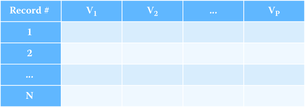
Figure 10.1: A typical rectangular data file format
The total error for this data set may be expressed by the following heuristic formula: \[\text{Total error } =\text{ Row error } + \text{ Column error } + \text{ Cell error}.\]
Row error
For the situations considered in this chapter, the row errors may be of three types:
Omissions: Some rows are missing, which implies that elements in the target population are not represented on the file.
Duplications: Some population elements occupy more than one row.
Erroneous inclusions: Some rows contain elements or entities that are not part of the target population.
Omissions:
For survey sample data sets, omissions include members of the target population that are either inadvertently or deliberately absent from the frame, as well as nonsampled frame members. For other types of data, the selectivity of the capture mechanism is a common cause of omissions. For example, a data set consisting of people who did a Google search in the past week can be used to make inferences about that specific population but if our goal was to make inferences about the larger population of internet users, this data set will exclude people who did not use Google Search. This selection bias can lead to inference errors if the people who did not use Google Search were different from those who did.
Such exclusions can therefore be viewed as a source of selectivity bias if inference is to be made about an even larger set of people, such as the general population. For one, persons who do not have access to the Internet are excluded from the data set. These exclusions may be biasing in that persons with Internet access may have quite different demographic characteristics from persons who do not have Internet access (Dutwin and Buskirk 2017). The selectivity of big data capture is similar to frame noncoverage in survey sampling and can bias inferences when researchers fail to consider it and compensate for it in their analyses.
Example: Google searches
As an example, in the United States, the word “Jewish” is included in 3.2 times more Google searches than “Mormon” (Stephens-Davidowitz and Varian 2015). This does not mean that the Jewish population is 3.2 times larger than the Mormon population. Other possible explanations could that Jewish people use the Internet in higher proportions, have more questions that require using the word “Jewish”, or there could be more searches for “Jewish food” food than “Mormon food.” Thus Google search data are more useful for relative comparisons than for estimating absolute levels.
A well-known formula in the survey literature provides a useful expression for the so-called coverage bias in the mean of some variable, \(V\). Denote the mean by \(\bar{V}\), and let \(\bar{V}_T\) denote the (possibly hypothetical because it may not be observable) mean of the target population of \(N_{T}\) elements, including the \(N_{T}-N\) elements that are missing from the observed data set. Then the bias due to this noncoverage is \(B_{NC} = \bar{V} - \bar{V}_T = (1 - N / N_T )(\bar{V}_C - \bar{V}_{NC})\), where \(\bar{V}_C\) is the mean of the covered elements (i.e., the elements in the observed data set) and \(\bar{V}_{NC}\) is the mean of the \(N_{T}-N\) noncovered elements. Thus we see that, to the extent that the difference between the covered and noncovered elements is large or the fraction of missing elements \((1 - N / N_T)\) is large, the bias in the descriptive statistic will also be large. As in survey research, often we can only speculate about the sizes of these two components of bias. Nevertheless, speculation is useful for understanding and interpreting the results of data analysis and cautioning ourselves regarding the risks of false inference.
Duplication:
We can also expect that big data sets, such as a data set containing Google searches during the previous week, could have the same person represented many times. People who conducted many searches during the data capture period would be disproportionately represented relative to those who conducted fewer searchers. If the rows of the data set correspond to tweets in a Twitter feed, duplication can arise when the same tweet is retweeted or when some persons are quite active in tweeting while others lurk and tweet much less frequently. Whether such duplications should be regarded as “errors” depends upon the goals of the analysis.
For example, if inference is to be made to a population of persons, persons who tweet multiple times on a topic would be overrepresented. If inference is to be made to the population of tweets, including retweets, then such duplication does not bias inference. This is also common in domains such as healthcare or human services where certain people have more interactions with the systems (medical appointments, consumption of social services, etc.) and can be over-represented when doing analysis at an individual interaction level.
When it is a problem, it still may not be possible to identify duplications in the data. Failing to account for them could generate duplication biases in the analysis. If these unwanted duplications can be identified, they can be removed from the data file (i.e., deduplication). Alternatively, if a certain number of rows, say \(d\), correspond to the same population unit, those row values can be weighted by \(1/d\) to correct the estimates for the duplications.
Erroneous inclusions:
Erroneous inclusions can also create biases. For example, Google searches or tweets may not be generated by a person but rather by a computer either maliciously or as part of an information-gathering or publicity-generating routine. Likewise, some rows may not satisfy the criteria for inclusion in an analysis—for example, an analysis by age or gender includes some row elements not satisfying the criteria. If the criteria can be applied accurately, the rows violating the criteria can be excluded prior to analysis. However, with big data, some out-of-scope elements may still be included as a result of missing or erroneous information, and these inclusions will bias inference.
Column error
The most common type of column error in survey data analysis is caused by inaccurate or erroneous labeling of the column data—an example of metadata error. In the TSE framework, this is referred to as a specification error. For example, a business register may include a column labeled “number of employees,” defined as the number of persons in the company who received a payroll check in the month preceding. Instead the column contains the number of persons on the payroll whether or not they received a check in the prior month, thus including, for example, persons on leave without pay.
When analyzing a more diverse set of data sources, such errors could happen because of the complexities involved in producing a data set. For example, data generated from an individual tweet may undergo a number of transformations before it is included in the analysis data set. This transformative process can be quite complex, involving parsing phrases, identifying words, and classifying them as to subject matter and then perhaps further classifying them as either positive or negative expressions about some phenomenon like the economy or a political figure. There is considerable risk of the resulting variables being either inaccurately defined or misinterpreted by the data analyst.
Example: Specification error with Twitter data
As an example, consider a Twitter data set where the rows correspond to tweets and one of the columns supposedly contains an indicator of whether the tweet contained one of the following key words: marijuana, pot, cannabis, weed, hemp, ganja, or THC. Instead, the indicator actually corresponds to whether the tweet contained a shorter list of words; say, either marijuana or pot. The mislabeled column is an example of specification error which could be a biasing factor in an analysis. For example, estimates of marijuana use based upon the indicator could be underestimates.
Cell errors
Finally, cell errors can be of three types: content error, specification error, or missing data.
Content Error: A content error occurs when the value in a cell satisfies the column definition but still deviates from the true value, whether or not the true value is known. For example, the value satisfies the definition of “number of employees” but is outdated because it does not agree with the current number of employees. Errors in sensitive data such as drug use, prior arrests, and sexual misconduct may be deliberate. Thus, content errors may be the result of the measurement process, a transcription error, a data processing error (e.g., keying, coding, editing), an imputation error, or some other cause.
Specification Error: Specification error is just as described for column error but applied to a cell. For example, the column is correctly defined and labeled; however, a few companies provided values that, although otherwise highly accurate, were nevertheless inconsistent with the required definition.
Missing data: Missing data, as the name implies, are just empty cells. As described in Kreuter and Peng (2014), data sets derived from big data are notoriously affected by all three types of cell error, particularly missing or incomplete data, perhaps because that is the most obvious deficiency.
Missing data can take two forms: missing information in a cell of a data matrix (referred to as item missingness) or missing rows (referred to as unit missingness), with the former being readily observable whereas the latter can be completely hidden from the analyst. Much is known from the survey research literature about how both types of missingness affect data analysis (see, for example, Little and Rubin (2014); Rubin (1976)). Rubin (1976) introduced the term missing completely at random (MCAR) to describe data where the data that are available (say, the rows of a data set) can be considered as a simple random sample of the inferential population (i.e., the population to which inferences from the data analysis will be made). Since the data set represents the population, MCAR data provide results that are generalizable to this population.
A second possibility also exists for the reasons why data are missing. For example, students who have high absenteeism may be missing because they were ill on the day of the test. They may otherwise be average performers on the test so, in this case, it has little to do with how they would score. Thus, the values are missing for reasons related to another variable, health, that may be available in the data set and completely observed. Students with poor health tend to be missing test scores, regardless of those student’s performance on the test. Rubin (1976) uses the term missing at random (MAR) to describe data that are missing for reasons related to completely observed variables in the data set. It is possible to compensate for this type of missingness in statistical inferences by modeling the missing data mechanism.
However, most often, missing data may be related to factors that are not represented in the data set and, thus, the missing data mechanism cannot be adequately modeled. For example, there may be a tendency for test scores to be missing from school administrative data files for students who are poor academic performers. Rubin calls this form of missingness nonignorable. With nonignorable missing data, the reasons for the missing observations depend on the values that are missing. When we suspect a nonignorable missing data mechanism, we need to use procedures much more complex than will be described here. Little and Rubin (2014) and Schafer (1997) discuss methods that can be used for nonignorable missing data. Ruling out a nonignorable response mechanism can simplify the analysis considerably.
In practice, it is quite difficult to obtain empirical evidence about whether or not the data are MCAR or MAR. Understanding the data generation process is invaluable for specifying models that appropriately represent the missing data mechanism and that will then be successful in compensating for missing data in an analysis. (Schafer and Graham Schafer and Graham (2002) provide a more thorough discussion of this issue.)
One strategy for ensuring that the missing data mechanism can be successfully modeled is to have available on the data set many variables that may be causally related to missing data. For example, features such as personal income are subject to high item missingness, and often the missingness is related to income. However, less sensitive, surrogate variables such as years of education or type of employment may be less subject to missingness. The statistical relationship between income and other income-related variables increases the chance that information lost in missing variables is supplemented by other completely observed variables. Model-based methods use the multivariate relationship between variables to handle the missing data. Thus, the more informative the data set, the more measures we have on important constructs, the more successfully we can compensate for missing data using model-based Approaches.
In the next section, we consider the impact of errors on some forms of analysis that are common in the big data literature. We will limit the focus on the effects of content errors on data analysis. However, there are numerous resources available for studying and mitigating the effects of missing data on analysis such as books by Little and Rubin (2014), Schafer (1997), and Allison (2001).
10.3 Example: Google Flu Trends
A well-known example of the risks of bad inference is provided by the Google Flu Trends series that uses Google searches on flu symptoms, remedies, and other related key words to provide near-real-time estimates of flu activity in the USA and 24 other countries84. Compared to CDC data, the Google Flu Trends provided remarkably accurate indicators of flu incidence in the USA between 2009 and 2011. However, for the 2012–2013 flu seasons, the Google Flu Trends estimates were almost double the CDC’s (Butler 2013). Lazer et al. (2014) cite two causes of this error: big data hubris and algorithm dynamics.
Hubris occurs when the big data researcher believes that the volume of the data compensates for any of its deficiencies, thus obviating the need for traditional, scientific analytic approaches. As Lazer et al. (2014) note, big data hubris fails to recognize that “quantity of data does not mean that one can ignore foundational issues of measurement and construct validity and reliability.”
Algorithm dynamics refers to properties of algorithms that allow them to adapt and “learn” as the processes generating the data change over time. Although explanations vary, the fact remains that Google Flu Trends estimates were too high and by considerable margins for 100 out of 108 weeks starting in July 2012. Lazer et al. (2014) also blame “blue team dynamics,” which arises when the data generating engine is modified in such a way that the formerly highly predictive search terms eventually failed to work. For example, when a Google user searched on “fever” or “cough,” Google’s other programs started recommending searches for flu symptoms and treatments—the very search terms the algorithm used to predict flu. Thus, flu-related searches artificially spiked as a result changes to the algorithm and the impact these changes had on user behavior. In survey research, this is similar to the measurement biases induced by interviewers who suggest to respondents who are coughing that they might have flu, then ask the same respondents if they think they might have flu.
Algorithm dynamic issues are not limited to Google. Platforms such as Twitter and Facebook are also frequently modified to improve the user experience. A key lesson provided by Google Flu Trends is that successful analyses using big data today may fail to produce good results tomorrow. All these platforms change their methodologies more or less frequently, with ambiguous results for any kind of long-term study unless highly nuanced methods are routinely used. Recommendation engines often exacerbate effects in a certain direction, but these effects are hard to tease out. Furthermore, other sources of error may affect Google Flu Trends to an unknown extent. For example, selectivity may be an important issue because the demographics of people with Internet access are quite different from the demographic characteristics related to flu incidence (Thompson, Comanor, and Shay 2006). Thus, the “at risk” population for influenza and the implied population based on Google searches do not correspond. This illustrates just one type of representativeness issue that often plagues big data analysis. In general it is an issue that algorithms are not (publicly) measured for accuracy, since they are often proprietary. Google Flu Trends is special in that it publicly failed. From what we have seen, most models fail privately and often without anyone noticing.
10.4 Errors in data analysis
The total error framework described above focuses on different types of errors in the data that can lead to incorrect inference. In addition to direct inference errors because of errors in the data, our analysis can also be incorrect because of these data errors. This section goes deeper into these common types of analysis errors when analyzing a diverse set of data sources. We begin by exploring errors that can happen under the assumption of accurate data and then go on to consider errors in three common types of analysis when data is not accurate: classification, correlation, and regression.
Analysis errors despite accurate data
Data deficiencies represent only one set of challenges for the big data analyst. Even if data is correct, other challenges can arise solely as a result of the massive size, rapid generation, and vast dimensionality of the data (Meng 2018). Fan et al. (2014) identify three issues—noise accumulation, spurious correlations, and incidental endogeneity—which will be discussed in this section. These issues should concern social scientists even if the data could be regarded as infallible. Content errors, missing data, and other data deficiencies will only exacerbate these problems.
Noise accumulation
To illustrate noise accumulation, Fan et al. (2014) consider the following scenario. Suppose an analyst is interested in classifying individuals into two categories, \(C_{1}\) and \(C_{2}\), based upon the values of 1,000 variables in a big data set. Suppose further that, unknown to the researcher, the mean value for persons in \(C_{1}\) is 0 on all 1,000 variables while persons in \(C_{2}\) have a mean of 3 on the first 10 variables and 0 on all other variables. Since we are assuming the data are error-free, a classification rule based upon the first \(m \le 10\) variables performs quite well, with little classification error. However, as more and more variables are included in the rule, classification error increases because the uninformative variables (i.e., the 990 variables having no discriminating power) eventually overwhelm the informative signals (i.e., the first 10 variables). In the Fan et al. (2014) example, when \(m > 200\), the accumulated noise exceeds the signal embedded in the first 10 variables and the classification rule becomes equivalent to a coin-flip classification rule.
Spurious correlations
High dimensionality can also introduce coincidental (or spurious) correlations in that many unrelated variables may be highly correlated simply by chance, resulting in false discoveries and erroneous inferences. The phenomenon depicted in Figure 10.2, is an illustration of this. Many more examples can be found on a website85 and in a book devoted to the topic (Vigen 2015). Fan et al. (2014) explain this phenomenon using simulated populations and relatively small sample sizes. They illustrate how, with 800 independent (i.e., uncorrelated) variables, the analyst has a 50% chance of observing an absolute correlation that exceeds 0.4. Their results suggest that there are considerable risks of false inference associated with a purely empirical approach to predictive analytics using high-dimensional data.
![An illustration of coincidental correlation between two variables: stork die-off linked to human birth decline [@sies1988new]](ChapterError/figures/fig10-3.png)
Figure 10.2: An illustration of coincidental correlation between two variables: stork die-off linked to human birth decline (Sies 1988)
Incidental Endogeneity
Finally, turning to incidental endogeneity, a key assumption in regression analysis is that the model covariates are uncorrelated with the residual error; endogeneity refers to a violation of this assumption. For high-dimensional models, this can occur purely by chance—a phenomenon Fan and Liao (2014) call incidental endogeneity. Incidental endogeneity leads to the modeling of spurious variation in the outcome variables resulting in errors in the model selection process and biases in the model predictions. The risks of incidental endogeneity increase as the number of variables in the model selection process grows large. Thus it is a particularly important concern for big data analytics.
Fan et al. (2014) as well as a number of other authors (Stock and Watson 2002; Fan, Samworth, and Wu 2009) (see, for example, Hall and Miller Hall and Miller (2009); Fan and Liao Fan and Liao (2012)) suggest robust statistical methods aimed at mitigating the risks of noise accumulation, spurious correlations, and incidental endogeneity. However, as previously noted, these issues and others are further compounded when data errors are present in a data set. Biemer and Trewin (1997) show that data errors will bias the results of traditional data analysis and inflate the variance of estimates in ways that are difficult to evaluate or mitigate in the analysis process.
10.4.1 Analysis errors resulting from inaccurate data
The previous sections examined some of the issues social scientists face as either \(N\) or \(p\) in Figure 10.1 becomes extremely large. When row, column, and cell errors are added into the mix, these problems can be further exacerbated. For example, noise accumulation can be expected to accelerate when random noise (i.e., content errors) afflicts the data. Spurious correlations that give rise to both incidental endogeneity and coincidental correlations can render correlation analysis meaningless if the error levels in big data are high. In this section, we consider some of the issues that arise in classification, correlation, and regression analysis as a result of content errors that may be either variable or systematic.
There are various important findings in this section. First, for rare classes, even small levels of error can impart considerable biases in classification analysis. Second, variable errors will attenuate correlations and regression slope coefficients; however, these effects can be mitigated by forming meaningful aggregates of the data and substituting these aggregates for the individual units in these analyses. Third, unlike random noise, systematic errors can bias correlation and regression analysis is unpredictable ways, and these biases cannot be effectively mitigated by aggregating the data. Finally, multilevel modeling can—under certain circumstances—be an important mitigation strategy for dealing with systematic errors emanating from multiple data sources. These issues will be examined in some detail in the remainder of this section.
We will start by focusing on two types of errors: variable (uncorrelated) errors and correlated errors. We’ll first describe these errors for continuous data and then extend it to categorical variables in the next section.
10.4.1.1 Variable (uncorrelated) and correlated error in continuous variables
Error models are essential for understanding the effects of error on data sets and the estimates that may be derived from them. They allow us to concisely and precisely communicate the nature of the errors that are being considered, the general conditions that give rise to them, how they affect the data, how they may affect the analysis of these data, and how their effects can be evaluated and mitigated. In the remainder of this chapter, we focus primarily on content errors and consider two types of error, variable errors and correlated errors, the latter a subcategory of systematic errors.
Variable errors are sometimes referred to as random noise or uncorrelated errors. For example, administrative databases often contain errors from a myriad of random causes, including mistakes in keying or other forms of data capture, errors on the part of the persons providing the data due to confusion about the information requested, difficulties in recalling information, the vagaries of the terms used to request the inputs, and other system deficiencies.
Correlated errors, on the other hand, carry a systematic effect that results in a nonzero covariance between the errors of two distinct units. For example, quite often, an analysis data set may combine multiple data sets from different sources and each source may impart errors that follow a somewhat different distribution. As we shall see, these differences in error distributions can induce correlated errors in the merged data set. It is also possible that correlated errors are induced from a single source as a result of different operators (e.g., computer programmers, data collection personnel, data editors, coders, data capture mechanisms) handling the data. Differences in the way these operators perform their tasks have the potential to alter the error distributions so that data elements handled by the same operator have errors that are correlated (Biemer and Lyberg 2003).
These concepts may be best expressed by a simple error model. Let \(y_{rc}\) denote the cell value for variable \(c\) on the \(r\)th unit in the data set, and let \(\varepsilon_{rc}\) denote the error associated with this value. Suppose it can be assumed that there is a true value underlying \(y_{rc}\), which is denoted by \(\mu_{rc}\). Then we can write \[\label{eq:10-1.1} y_{rc} = \mu_{rc} + \varepsilon_{rc}.\]
At this point, \(\varepsilon_{rc}\) is not stochastic in nature because a statistical process for generating the data has not yet been assumed. Therefore, it is not clear what correlated error really means. To remedy this problem, we can consider the hypothetical situation where the processes generating the data set can be repeated under the same general conditions (i.e., at the same point in time with the same external and internal factors operating). Each time the processes are repeated, a different set of errors may be realized. Thus, it is assumed that although the true values, \(\mu_{rc}\), are fixed, the errors, \(\varepsilon_{rc}\), can vary across the hypothetical, infinite repetitions of the data set generating process. Let \(\mbox{E}(\cdot)\) denote the expected value over all these hypothetical repetitions, and define the variance, \(\mathrm{Var}(\cdot)\), and covariance, \(\mathrm{Cov}(\cdot)\), analogously.
For the present, error correlations between variables are not considered, and thus the subscript, \(c\), is dropped to simplify the notation. For the uncorrelated data model, we assume that \({\rm E}(y_r \vert r) = \mu_r\), \({\rm Var}(y_r \vert r) = \sigma_\varepsilon^2\), and \({\rm Cov}(y_r ,y_s \vert r,s) = 0\), for \(r \ne s\). For the correlated data model, the latter assumption is relaxed. To add a bit more structure to the model, suppose the data set is the product of combining data from multiple sources (or operators) denoted by \(j = 1, 2, \ldots, J\), and let \(b_j\) denote the systematic effect of the \(j\)th source. Here we also assume that, with each hypothetical repetition of the data set generating process, these systematic effects can vary stochastically. (It is also possible to assume the systematic effects are fixed. See, for example, Biemer and Stokes (1991) for more details on this model.) Thus, we assume that \({\rm E}(b_j ) = 0\), \({\rm Var}(b_j ) = \sigma_b^2\), and \({\rm Cov}(b_j ,b_k ) = 0\) for \(j \ne k\).
Finally, for the \(r\)th unit within the \(j\)th source, let \(\varepsilon_{rj} = b_j + e_{rj}\). Then it follows that \[\label{eq:10-1.2} \begin{array}{lcl@{\quad}l} \mathrm{Cov}(\varepsilon_{rj} ,\varepsilon_{sk}) = \begin{cases} \sigma_b^2 + \sigma_\varepsilon^2 & \text{for } r = s,j = k, \\ %& =& \sigma_\varepsilon^2&\text{for } r = s,j \ne k, \\ % &=& 0 & \text{for } r \ne s,j \ne k. \end{cases} \end{array}\] The case where \(\sigma_b^2 = 0\) corresponds to the uncorrelated error model (i.e., \(b_j = 0\)) and thus \(\varepsilon_{rj}\) is purely random noise.
Example: Speed sensor
Suppose that, due to calibration error, the \(j\)th speed sensor in a traffic pattern study underestimates the speed of vehicle traffic on a highway by an average of 4 miles per hour. Thus, the model for this sensor is that the speed for the \(r\)th vehicle recorded by this sensor \((y_{rj})\) is the vehicle’s true speed \((\mu_{rj})\) minus 4 mph (\(b_{j}\)) plus a random departure from \(-4\) for the \(r\)th vehicle (\(\varepsilon_{rj}\)). Note that to the extent that \(b_{j}\) varies across sensors \(j = 1,\ldots ,J\) in the study, \(\sigma_b^2\) will be large. Further, to the extent that ambient noise in the readings for \(j\)th sensor causes variation around the values \(\mu_{rc} + b_j\), then \(\sigma_\varepsilon^2\) will be large. Both sources of variation will reduce the reliability of the measurements. However, as shown in Section Errors in Correlation analysis, the systematic error component is particularly problematic for many types of analysis.
10.4.1.2 Extending Variable and Correlated Error to Categorical Data
For variables that are categorical, the model of the previous section is not appropriate because the assumptions it makes about the error structure do not hold. For example, consider the case of a binary (\(0/1\)) variable. Since both \(y_r\) and \(\mu_r\) should be either 1 or 0, the error in equation (10.1) must assume the values of \(-1\), \(0\), or \(1\). A more appropriate model is the misclassification model described by Biemer (2011), which we summarize here.
Let \(\phi_r\) denote the probability of a false positive error (i.e., \(\phi_r = \Pr (y_r = 1\vert \mu_r = 0)\)), and let \(\theta_r\) denote the probability of a false negative error (i.e., \(\theta_r =\Pr (y_r = 0\vert \mu_r = 1)\)). Thus, the probability that the value for row \(r\) is correct is \(1 - \theta_r\) if the true value is \(1\), and \(1 - \phi_r\) if the true value is \(0\).
As an example, suppose an analyst wishes to compute the proportion, \(P = \sum_r {y_r / N}\), of the units in the file that are classified as \(1\), and let \(\pi = \sum_r {\mu_r / N}\) denote the true proportion. Then under the assumption of uncorrelated error, Biemer (2011) shows that \[\label{eq:10-1.3} P = \pi (1 - \theta ) + (1 - \pi )\phi,\] where \(\theta = \sum_r {\theta_r / N}\) and \(\phi = \sum_r {\phi_r / N}\).
In the classification error literature, the sensitivity of a classifier is defined as \(1 - \theta\), that is, the probability that a true positive is correctly classified. Correspondingly, \(1 - \phi\) is referred to as the specificity of the classifier, that is, the probability that a true negative is correctly classified. Two other quantities that will be useful in our study of misclassification error are the positive predictive value (PPV) and negative predictive value (NPV) given by \[\label{eq:10-1.4} \mathrm{PPV} = \Pr (\mu_r = 1\vert y_r = 1),\quad\mathrm{NPV} = \Pr (\mu_r = 0\vert y_r = 0).\] The PPV (NPV) is the probability that a positive (negative) classification is correct.
10.4.1.3 Errors when analyzing rare population groups
One of the attractions of newer sources of data such as social media is the ability to study rare population groups that seldom show up in large enough numbers in designed studies such as surveys and clinical trials. While this is true in theory, in practice content errors can affect the inferences that can be drawn from this data. We illustrate this using the following contrived and somewhat amusing example. The results in this section are particularly relevant to the approaches considered in Chapter Machine Learning.
Example: Thinking about probabilities
Suppose, using big data and other resources, we construct a terrorist detector and boast that the detector is 99.9% accurate. In other words, both the probability of a false negative (i.e., classifying a terrorist as a nonterrorist, \(\theta\)) and the probability of a false positive (i.e., classifying a nonterrorist as a terrorist, \(\phi\)) are 0.001. Assume that about \(1\) person in a million in the population is a terrorist, that is, \(\pi = 0.000001\) (hopefully, somewhat of an overestimate). Your friend, Terry, steps into the machine and, to Terry’s chagrin (and your surprise) the detector declares that he is a terrorist! What are the odds that the machine is right? The surprising answer is only about 1 in 1000. That is, 999 times out of 1,000 times the machine classifies a person as a terrorist, the machine will be wrong!
How could such an accurate machine be wrong so often in the terrorism example? Let us do the math.
The relevant probability is the PPV of the machine: given that the machine classifies an individual (Terry) as a terrorist, what is the probability the individual is truly a terrorist? Using the notation in Section Extending Variable and Correlated Error to Categorical Data and Bayes’ rule, we can derive the PPV as \[\begin{aligned} \Pr (\mu_r = 1\vert y_r = 1) &= \frac{\Pr (y_r = 1\vert \mu_r = 1)\Pr(\mu_r = 1)}{\Pr (y_r = 1)} \\ &= \frac{(1 - \theta )\pi }{\pi (1 - \theta ) + (1 - \pi )\phi } \\ &= \frac{0.999\times 0.000001}{0.000001\times 0.999 + 0.99999\times 0.001} \\ &\approx 0.001.\end{aligned}\]
This example calls into question whether security surveillance using emails, phone calls, etc. can ever be successful in finding rare threats such as terrorism since to achieve a reasonably high PPV (say, 90%) would require a sensitivity and specificity of at least \(1-10^{-7}\), or less than 1 chance in 10 million of an error.
To generalize this approach, note that any population can be regarded as a mixture of subpopulations. Mathematically, this can be written as \[\label{eq:10-1.5} f(y\vert \mathbf{x};{\boldsymbol \eth}) = \pi_1 f(y\vert \mathbf{x};\eth_1 ) + \pi_2 f(y\vert \mathbf{x};\eth_2 ) + \ldots + \pi_K f(y\vert \mathbf{x};\eth_K ),\] where \(f(y\vert \mathbf{x}; {\boldsymbol \theta})\) denotes the population distribution of \(y\) given the vector of explanatory variables \(\mathbf{x}\) and the parameter vector \({\boldsymbol \theta } = (\theta_1 ,\theta_2, \ldots, \theta_K )\), \(\pi _k\) is the proportion of the population in the \(k\)th subgroup, and \(f(y\vert \mathbf{x};\theta_k)\) is the distribution of \(y\) in the \(k\)th subgroup. A rare subgroup is one where \(\pi_k\) is quite small (say, less than 0.01).
Table 10.1 shows the PPV for a range of rare subgroup sizes when the sensitivity is perfect (i.e., no misclassification of true positives) and specificity is not perfect but still high. This table reveals the fallacy of identifying rare population subgroups using fallible classifiers unless the accuracy of the classifier is appropriately matched to the rarity of the subgroup. As an example, for a 0.1% subgroup, the specificity should be at least 99.99%, even with perfect sensitivity, to attain a 90% PPV.
| \(\pi_k\) | Specificity | ||
|---|---|---|---|
| 99% | 99.9% | 99.99% | |
| 0.1 | 91.70 | 99.10 | 99.90 |
| 0.01 | 50.30 | 91.00 | 99.00 |
| 0.001 | 9.10 | 50.00 | 90.90 |
| 0.0001 | 1.00 | 9.10 | 50.00 |
10.4.1.4 Errors in Correlation analysis
In Section Errors in data analysis, we considered the problem of incidental correlation that occurs when an analyst correlates pairs of variables selected from big data stores containing thousands of variables. In this section, we discuss how errors in the data can exacerbate this problem or even lead to failure to recognize strong associations among the variables. We confine the discussion to the continuous variable model of Section Variable (uncorrelated) and correlated error in continuous variables and begin with theoretical results that help explain what happens in correlation analysis when the data are subject to variable and systematic errors.
For any two variables in the data set, \(c\) and \(d\), define the covariance between \(y_{rc}\) and \(y_{rd}\) as \[\label{eq:10-1.6} \sigma_{y\vert cd} = \frac{\sum\nolimits_r {\mbox{E}(y_{rc} - \bar{y}_c )(y_{rd} - \bar {y}_d )} }{N},\] where the expectation is with respect to the error distributions and the sum extends over all rows in the data set. Let \[\sigma_{\mu \vert cd} = \frac{\sum\nolimits_r {(\mu_{rc} - \bar{\mu }_c } )(\mu_{rd} - \bar{\mu }_d )}{N}\] denote the population covariance. (The population is defined as the set of all units corresponding to the rows of the data set.) For any variable \(c\), define the variance components \[\sigma_{y\vert c}^2 = \frac{\sum_r {(y_{rc} - \bar{y}_c )^2}}{N},\quad \sigma_{\mu \vert c}^2 =\frac{% \sum_r {(\mu_{rc} - \bar {\mu }_c } )^2}{N},\] and let \[R_c = \frac{\sigma_{\mu \vert c}^2}{\sigma_{\mu \vert c}^2 + \sigma_{b\vert c}^2 + \sigma_{\varepsilon \vert c}^2},\quad \rho_c = \frac{\sigma_{b\vert c}^2}{\sigma_{\mu \vert c}^2 + \sigma_{b\vert c}^2 + \sigma _{\varepsilon \vert c}^2},\] with analogous definitions for \(d\). The ratio \(R_{c}\) is known as the reliability ratio, and \(\rho_c\) will be referred to as the intra-source correlation. Note that the reliability ratio is the proportion of total variance that is due to the variation of true values in the data set. If there were no errors, either variable or systematic, then this ratio would be 1. To the extent that errors exist in the data, \(R_{c}\) will be less than 1.
Likewise, \(\rho_c\) is also a ratio of variance components that reflects the proportion of total variance that is due to systematic errors with biases that vary by data source. A value of \(\rho_c\) that exceeds 0 indicates the presence of systematic error variation in the data. As we shall see, even small values of \(\rho_c\) can cause big problems in correlation analysis.
Using the results in Biemer and Trewin (1997), it can be shown that the correlation between \(y_{rc}\) and \(y_{rd}\), defined as \(\rho_{y\vert cd} = \sigma_{y\vert cd} / \sigma_{y\vert c} \sigma_{y\vert d}\), can be expressed as \[\label{eq:10-1.7} \rho_{y\vert cd} = \sqrt {R_c R_d } \rho_{\mu \vert cd} + \sqrt {\rho_c \rho_d }.\] Note that if there are no errors (i.e., when \(\sigma_{b\vert c}^2 = \sigma_{\varepsilon \vert c}^2 = 0\)), then \(R_c = 1\), \(\rho_c =0\), and the correlation between \(y_{c}\) and \(y_{d}\) is just the population correlation.
Let us consider the implications of these results first without systematic errors (i.e., only variable errors) and then with the effects of systematic errors.
Variable errors only
If the only errors are due to random noise, then the additive term on the right in equation (10.2) is 0 and \(\rho_{y\vert cd} = \sqrt {R_c R_d } \rho _{\mu \vert cd}\), which says that the correlation is attenuated by the product of the root reliability ratios. For example, suppose \(R_c = R_d = 0.8\), which is considered excellent reliability. Then the observed correlation in the data will be about 80% of the true correlation; that is, correlation is attenuated by random noise. Thus, \(\sqrt {R_c R_d }\) will be referred to as the attenuation factor for the correlation between two variables.
Quite often in the analysis of big data, the correlations being explored are for aggregate measures, as in Figure 10.2. Therefore, suppose that, rather than being a single element, \(y_{rc}\) and \(y_{rd}\) are the means of \(n_{rc}\) and \(n_{rd}\) independent elements, respectively. For example, \(y_{rc}\) and \(y_{rd}\) may be the average rate of inflation and the average price of oil, respectively, for the \(r\)th year, for \(r = 1,\ldots ,N\) years. Aggregated data are less affected by variable errors because, as we sum up the values in a data set, the positive and negative values of the random noise components combine and cancel each other under our assumption that \(\mathrm{E}(\varepsilon_{rc} ) = 0\). In addition, the variance of the mean of the errors is of order \(O(n_{rc}^{ - 1} )\).
To simplify the result for the purposes of our discussion, suppose \(n_{rc} = n_c\), that is, each aggregate is based upon the same sample size. It can be shown that equation (10.2) still applies if we replace \(R_c\) by its aggregated data counterpart denoted by \(R_c^A = \sigma_{\mu \vert c}^2 / (\sigma_{\mu \vert c}^2 + \sigma_{\varepsilon \vert c}^2 / n_c )\). Note that \(R_c^A\) converges to 1 as \(n_c\) increases, which means that \(\rho _{y\vert cd}\) will converge to \(\rho_{\mu \vert cd}\). Figure 10.3 illustrates the speed at which this convergence occurs.
In this figure, we assume \(n_c = n_d = n\) and vary \(n\) from 0 to 60. We set the reliability ratios for both variables to 0.5 (which is considered to be a “fair” reliability) and assume a population correlation of \(\rho_{\mu \vert cd} = 0.5\). For \(n\) in the range \([2,10]\), the attenuation is pronounced. However, above 10 the correlation is quite close to the population value. Attenuation is negligible when \(n > 30\). These results suggest that variable error can be mitigated by aggregating like elements that can be assumed to have independent errors.
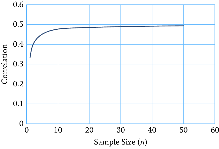
Figure 10.3: Correlation as a function of sample size (I)
Both variable and systematic errors
If both systematic and variable errors contaminate the data, the additive term on the right in equation (10.2) is positive. For aggregate data, the reliability ratio takes the form \[\label{eq:10-1.8} R_c^A = \frac{{\sigma_{\mu |c}^2}}{{\sigma_{\mu |c}^2 + \sigma _{b|c}^2 + n_c^{ - 1}\sigma_{\varepsilon |c}^2}},\] which converges not to 1 as in the case of variable error only, but to \(\sigma_{\mu \vert c}^2 / (\sigma_{\mu \vert c}^2 + \sigma_{b\vert c}^2)\), which will be less than 1. Thus, some attenuation is possible regardless of the number of elements in the aggregate. In addition, the intra-source correlation takes the form \[\label{eq:10-1.9} \rho_c^A = \frac{{\sigma_{b|c}^2}}{{\sigma_{\mu |c}^2 + \sigma_{b|c}^2 + n_c^{ - 1}\sigma_{\varepsilon |c}^2}},\] which converges to \(\rho_c^A = \sigma_{b|c}^2/(\sigma_{\mu |c}^2 + \sigma _{b|c}^2)\), or approximately to \(1 - R_c^A\) for large \(n_c\). Thus, the systematic effects may still adversely affect correlation analysis without regard to the number of elements comprising the aggregates.
For example, consider the illustration in Figure 10.3 with \(n_c = n_d = n\), reliability ratios (excluding systematic effects) set at \(0.5\) and population correlation at \(\rho_{\mu \vert cd} = 0.5\). In this scenario, let \(\rho_c = \rho_d = 0.25\). Figure 10.4 shows the correlation as a function of the sample size with systematic errors compared to the correlation without systematic errors. Correlation with systematic errors is both inflated and attenuated. However, at the assumed level of intra-source variation, the inflation factor overwhelms the attenuation factors and the result is a much inflated value of the correlation across all aggregate sizes.
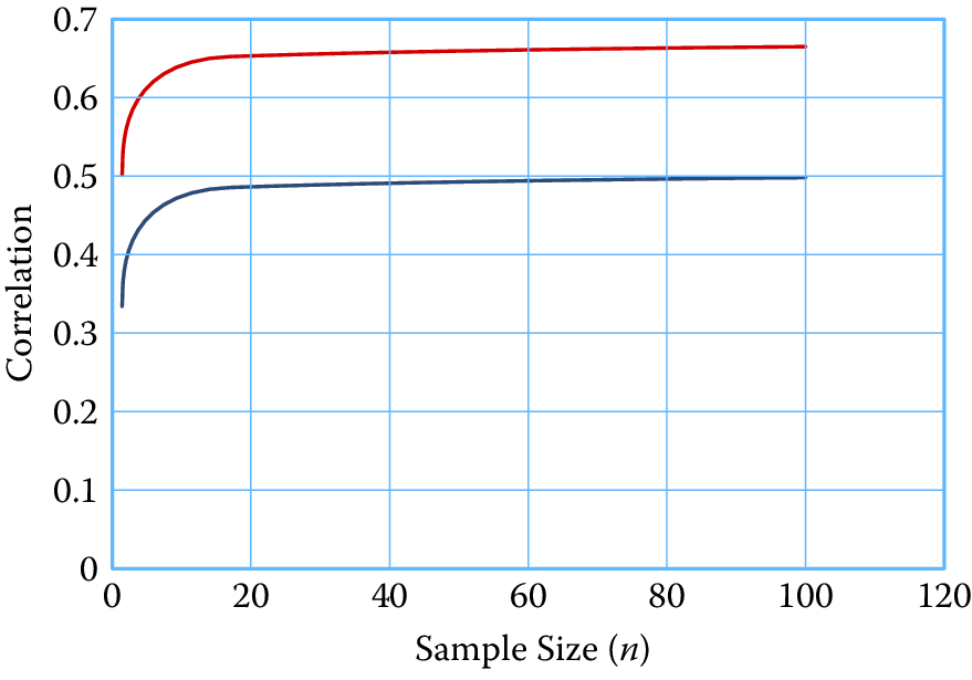
Figure 10.4: Correlation as a function of sample size (II)
To summarize these findings, correlation analysis is attenuated by variable errors, which can lead to null findings when conducting a correlation analysis and the failure to identify associations that exist in the data. Combined with systematic errors that may arise when data are extracted and combined from multiple sources, correlation analysis can be unpredictable because both attenuation and inflation of correlations can occur. Aggregating data mitigates the effects of variable error but may have little effect on systematic errors.
10.4.1.5 Errors in Regression analysis
The effects of variable errors on regression coefficients are well known (Cochran 1968; Fuller 1991; Biemer and Trewin 1997). The effects of systematic errors on regression have been less studied. We review some results for both types of errors in this section.
Consider the simple situation where we are interested in computing the population slope and intercept coefficients given by \[\label{eq:10-1.10} b = \frac{\sum_r {(y_r - \bar{y})(x_r - \bar{x})} }{\sum_r {(x_r - \bar{x})^2} }\quad\mbox{and}\quad b_0 = \bar{y} - b\bar{x},\] where, as before, the sum extends over all rows in the data set. When \(x\) is subject to variable errors, it can be shown that the observed regression coefficient will be attenuated from its error-free counterpart. Let \(R_x\) denote the reliability ratio for \(x\). Then \[\label{eq:10-1.11} b = R_x B,\] where \(B = \sum_r {(y_r - \bar{y})(\mu_{r\vert x} - \bar{\mu }_x )} / \sum_r {(\mu_{r\vert x} - \bar{\mu }_x )^2}\) is the population slope coefficient, with \(x_r = \mu_{r\vert x} + \varepsilon_{r\vert x}\), where \(\varepsilon_{r\vert x}\) is the variable error with mean 0 and variance \(\sigma_{\varepsilon\vert x}^2\). It can also be shown that \(\mbox{Bias}(b_0 ) \approx B(1 - R_x )\bar{\mu }_x\).
As an illustration of these effects, consider the regressions displayed in Figure 10.5, which are based upon contrived data. The regression on the left is the population (true) regression with a slope of \(1.05\) and an intercept of \(-0.61\). The regression on the left uses the same \(y\)- and \(x\)-values. The only difference is that normal error was added to the \(x\)-values, resulting in a reliability ratio of \(0.73\). As the theory predicted, the slope was attenuated toward \(0\) in direct proportion to the reliability, \(R_{x}\). As random error is added to the \(x\)-values, reliability is reduced and the fitted slope will approach \(0\).
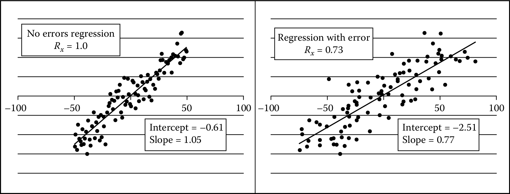
Figure 10.5: Regression of y on x with and without variable error. On the left is the population regression with no error in the x variable. On the right, variable error was added to the x-values with a reliability ratio of 0.73. Note its attenuated slope, which is very near the theoretical value of 0.77
When the dependent variable, \(y\), only is subject to variable error, the regression deteriorates, but the expected values of the slope and intercept coefficients are still equal to true to their population values. To see this, suppose \(y_r = \mu_{y\vert r} + \varepsilon_{y\vert r}\), where \(\mu_{r\vert y}\) denotes the error-free value of \(y_r\) and \(\varepsilon_{r\vert y}\) is the associated variable error with variance \(\sigma _{\varepsilon \vert y}^2\). The regression of \(y\) on \(x\) can now be rewritten as \[\label{eq:10-1.12} \mu_{y\vert r} = b_0 + bx_r + e_r - \varepsilon _{r\vert y},\] where \(e_r\) is the usual regression residual error with mean \(0\) and variance \(\sigma_e^2\), which is assumed to be uncorrelated with \(\varepsilon_{r\vert y}\). Letting \({e}' = e_r - \varepsilon_{r\vert y}\), it follows that the regression in equation (10.3) is equivalent to the previously considered regression of \(y\) on \(x\) where \(y\) is not subject to error, but now the residual variance is increased by the additive term, that is, \(\sigma_{e}^{\prime2} = \sigma_{\varepsilon \vert y}^2 + \sigma_e^2\).
Chai (1971) considers the case of systematic errors in the regression variables that may induce correlations both within and between variables in the regression. He shows that, in the presence of systematic errors in the independent variable, the bias in the slope coefficient may either attenuate the slope or increase its magnitude in ways that cannot be predicted without extensive knowledge of the error properties. Thus, like the results from correlation analysis, systematic errors greatly increase the complexity of the bias effects and their effects on inference can be quite severe.
One approach for dealing with systematic error at the source level in regression analysis is to model it using, for example, random effects (Hox 2010). In brief, a random effects model specifies \(y_{ijk} = \beta_{0i}^\ast + \beta x_{ijk} + \varepsilon_{ijk}\), where \({\varepsilon }'_{ijk} = b_i + \varepsilon_{ijk}\) and \(\mathrm{Var}({\varepsilon }'_{ijk} ) = \sigma_b^2 + \sigma_{\varepsilon \vert j}^2\). The next section considers other mitigation strategies that attempt to eliminate the error rather than model it.
10.5 Detecting and Compensating for Data Errors
For survey data and other designed data collections, error mitigation86 begins at the data generation stage by incorporating design strategies that generate high-quality data that are at least adequate for the purposes of the data users. For example, missing data can be mitigated by repeated follow-up of nonrespondents, questionnaires can be perfected through pretesting and experimentation, interviewers can be trained in the effective methods for obtaining highly accurate responses, and computer-assisted interviewing instruments can be programmed to correct errors in the data as they are generated. For data where the data generation process is often outside the purview of the data collectors, as noted in Section Introduction, there is limited opportunity to address deficiencies in the data generation process. Instead, error mitigation must necessarily begin at the data processing stage. We illustrate this error mitigation process using two types of techniques—data editing and cleaning.
Data editing is a set of methodologies for identifying and correcting (or transforming) anomalies in the data. It often involves verifying that various relationships among related variables of the data set are plausible and, if they are not, attempting to make them so. Editing is typically a rule-based approach where rules can apply to a particular variable, a combination of variables, or an aggregate value that is the sum over all the rows or a subset of the rows in a data set. Recently, data mining and machine learning techniques have been applied to data editing with excellent results (see Chandola et al. Chandola, Banerjee, and Kumar (2009) for a review). Tree-based methods such as classification and regression trees and random forests are particularly useful for creating editing rules for anomaly identification and resolution (Petrakos et al. 2004). However, some human review may be necessary to resolve the most complex situations.
For larger amounts of data, the identification of data anomalies could result in possibly billions of edit failures. Even if only a tiny proportion of these required some form of manual review for resolution, the task could still require the inspection of tens or hundreds of thousands of query edits, which would be infeasible for most applications. Thus, micro-editing must necessarily be a completely automated process unless it can be confined to a relatively small subset of the data. As an example, a representative (random) subset of the data set could be edited using manual editing for purposes of evaluating the error levels for the larger data set, or possibly to be used as a training data set, benchmark, or reference distribution for further processing, including recursive learning.
To complement fully automated micro-editing, data editing involving large amounts of data usually involves top-down or macro-editing approaches. For such approaches, analysts and systems inspect aggregated data for conformance to some benchmark values or data distributions that are known from either training data or prior experience. When unexpected or suspicious aggregates are identified, the analyst can “drill down” into the data to discover and, if possible, remove the discrepancy by either altering the value at the source (usually a micro-data element) or delete the edit-failed value.
There are a variety of methods that may be effective in macro-editing. Some of these are based upon data mining (Natarajan, Li, and Koronios 2010), machine learning (Clarke 2014), cluster analysis (Duan et al. 2009; He, Xu, and Deng 2003), and various data visualization tools such as treemaps (Johnson and Shneiderman 1991; Shneiderman 1992; Tennekes and Jonge 2011) and tableplots (Tennekes, Jonge, and Daas 2013; Puts, Daas, and Waal 2015; Tennekes, Jonge, and Daas 2012). We further explore tableplots below.
10.5.1 TablePlots
Like other visualization techniques examined in Chapter Information Visualization, the tableplot has the ability to summarize a large multivariate data set in a single plot (Malik, Unwin, and Gribov 2010). In editing data, it can be used to detect outliers and unusual data patterns. Software for implementing this technique has been written in R and is available from the Comprehensive R Archive Network (https://cran.r-project.org/) (R Core Team 2013). Figure 10.6 shows an example. The key idea is that micro-aggregates of two related variables should have similar data patterns. Inconsistent data patterns may signal errors in one of the aggregates that can be investigated and corrected in the editing process to improve data quality. The tableplot uses bar charts created for the micro-aggregates to identify these inconsistent data patterns.
Each column in the tableplot represents some variable in the data table, and each row is a “bin” containing a subset of the data. A statistic such as the mean or total is computed for the values in a bin and is displayed as a bar (for continuous variables) or as a stacked bar for categorical variables.
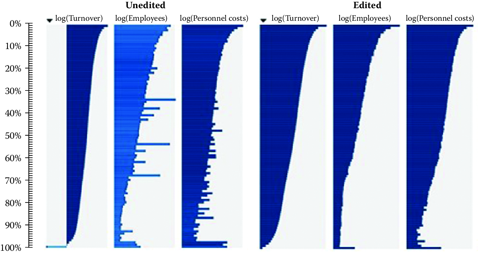
Figure 10.6: Comparison of tableplots for the Dutch Structural Business Statistics Survey for five variables before and after editing. Row bins with high missing and unknown numeric values are represented by lighter colored bars
The sequence of steps typically involved in producing a tableplot is as follows:
Sort the records in the data set by the key variable.
Divide the sorted data set into \(B\) bins containing the same number of rows.
For continuous variables, compute the statistic to be compared across variables for each row bin, say \(T_{b}\), for \(b = 1,\ldots ,B\), for each continuous variable, \(V\), ignoring missing values. The level of missingness for \(V\) may be represented by the color or brightness of the bar. For categorical variables with \(K\) categories, compute the proportion in the \(k\)th category, denoted by \(P_{bk}\). Missing values are assigned to a new (\(K+1\))th category (“missing”).
For continuous variables, plot the \(B\) values \(T_{b}\) as a bar chart. For categorical variables, plot the \(B\) proportions \(P_{bk}\) as astacked bar chart.
Typically, \(T_{b}\) is the mean, but other statistics such as the median or range could be plotted if they aid in the outlier identification process. For highly skewed distributions, Tennekes and de Jonge (2011) suggest transforming \(T_{b}\) by the log function to better capture the range of values in the data set. In that case, negative values can be plotted as \(\log(-T_{b})\) to the left of the origin and zero values can be plotted on the origin line. For categorical variables, each bar in the stack should be displayed using contrasting colors so that the divisions between categories are apparent.
Tableplots appear to be well suited for studying the distributions of variable values, the correlation between variables, and the occurrence and selectivity of missing values. Because they can help visualize massive, multivariate data sets, they seem particularly well suited for big data. Currently, the R implementation of tableplot is limited to \(2\) billion records.
The tableplot in Figure 10.6 is taken from Tennekes and de Jonge (2011) for the annual Dutch Structural Business Statistics survey, a survey of approximately 58,000 business units annually. Topics covered in the questionnaire include turnover, number of employed persons, total purchases, and financial results. Figure 10.6 was created by sorting on the first column, viz., log(turnover), and dividing the 57,621 observed units into 100 bins, so that each row bin contains approximately 576 records. To aid the comparisons between unedited and edited data, the two tableplots are displayed side by side, with the unedited graph on the left and the edited graph on the right. All variables were transformed by the log function.
The unedited tableplot reveals that all four of the variables in the comparison with log(turnover) show some distortion by large values for some row bins. In particular, log(employees) has some fairly large nonconforming bins with considerable discrepancies. In addition, that variable suffers from a large number of missing values, as indicated by the brightness of the bar color. All in all, there are obvious data quality issues in the unprocessed data set for all four of these variables that should be dealt with in the subsequent processing steps.
The edited tableplot reveals the effect of the data checking and editing strategy used in the editing process. Notice the much darker color for the number of employees for the graph on the left compared to same graph on the right. In addition, the lack of data in the lowest part of the turnover column has been somewhat improved. The distributions for the graph on the right appear smoother and are less jagged.
10.6 Summary
As social scientists, we are deeply concerned with making sure that the inferences we make from our analysis are valid. Since many of the newer data sources we are using are not collected or generated from instruments and methods designed to produce valid and reliable data for scientific analysis and discovery, they can lead to inference errors. This chapter described different types of errors that we encounter to make us aware of these limitations and take the necessary steps to understand and hopefully mitigate the effects of hidden errors on our results.
In addition to describing the types of errors, this chapter also gives an example of a solution to clean up the data before analysis. Another option that was not discussed is the possibility of using analytical techniques that attempt to model errors and compensate for them in the analysis. Such techniques include the use of latent class analysis for classification error (Biemer 2011), multilevel modeling of systematic errors from multiple sources (Hox 2010), and Bayesian statistics for partitioning massive data sets across multiple machines and then combining the results (Ibrahim and Chen 2000; Scott et al. 2013).
While this chapter has focused on the accuracy of the data and the validity of the inference, other data quality dimensions such as timeliness, comparability, coherence, and relevance that we have not considered in this chapter are also important. For example, timeliness often competes with accuracy because achieving acceptable levels of the latter often requires greater expenditures of resources and time. In fact, some applications of data analysis prefer results that are less accurate for the sake of timeliness. Biemer and Lyberg (2003) discuss these and other issues in some detail.
It is important to understand that we will rarely, if ever, get perfect data for our analysis. Every data source will have some limitation—some will be inaccurate, some will become stale, and some will have sample bias. The key is to 1) be aware of the limitations of each data source, 2) incorporate that awareness in to the analysis that is being done with it, and 3) understand what type of inference errors it can lead to in order to appropriately communicate the results and make sound decisions.
10.7 Resources
The American Association of Public Opinion Research has a number of resources on its website.87 See, in particular, its report on big data (Japec et al. 2015).
The Journal of Official Statistics88 is a standard resource with many relevant articles. There is also an annual international conference (International Total Survey Error Workshop) on the total survey error framework, supported by major survey organizations.
The Errors and Inference workbook of Chapter Workbooks provides an introduction to sensitivity analysis and imputation.89
References
Allison, Paul D. 2001. Missing Data. Sage Publications.
Biemer, Paul P. 2010. “Total Survey Error: Design, Implementation, and Evaluation.” Public Opinion Quarterly 74 (5). AAPOR: 817–48.
Biemer, Paul P. 2011. Latent Class Analysis of Survey Error. John Wiley & Sons.
Biemer, Paul P., and Lars E. Lyberg. 2003. Introduction to Survey Quality. John Wiley & Sons.
Biemer, Paul P., and S. Lynne Stokes. 1991. “Approaches to Modeling Measurement Error.” In Measurement Errors in Surveys, edited by Paul P. Biemer, Robert M. Groves, Lars E. Lyberg, Nancy A. Mathiowetz, and Seymour Sudman, 54–68. John Wiley.
Biemer, Paul P., and Dennis Trewin. 1997. “A Review of Measurement Error Effects on the Analysis of Survey Data.” In Survey Measurement and Process Quality, edited by Lars Lyberg, Paul P. Biemer, Martin Collins, Edith De Leeuw, Cathryn Dippo, Norbert Schwarz, and Dennis Trewin, 601–32. John Wiley & Sons.
Butler, Declan. 2013. “When Google Got Flu Wrong.” Nature 494 (7436): 155.
Chandola, Varun, Arindam Banerjee, and Vipin Kumar. 2009. “Anomaly Detection: A Survey.” ACM Computing Surveys 41 (3).
Clarke, Claire. 2014. “Editing Big Data with Machine Learning Methods.” Paper presented at the Australian Bureau of Statistics Symposium, Canberra.
Cochran, William G. 1968. “Errors of Measurement in Statistics.” Technometrics 10 (4). Taylor & Francis Group: 637–66.
Duan, Lian, Lida Xu, Ying Liu, and Jun Lee. 2009. “Cluster-Based Outlier Detection.” Annals of Operations Research 168 (1). Springer: 151–68.
Dutwin, David, and Trent D. Buskirk. 2017. “Reply.” Public Opinion Quarterly 81 (S1): 246–49.
Fan, Jianqing, and Yuan Liao. 2012. “Endogeneity in Ultrahigh Dimension.” Princeton University.
Fan, Jianqing, and Yuan Liao. 2014. “Endogeneity in High Dimensions.” Annals of Statistics 42 (3): 872.
Fan, Jianqing, Fang Han, and Han Liu. 2014. “Challenges of Big Data Analysis.” National Science Review 1 (2). Oxford University Press: 293–314.
Fan, Jianqing, Richard Samworth, and Yichao Wu. 2009. “Ultrahigh Dimensional Feature Selection: Beyond the Linear Model.” Journal of Machine Learning Research 10: 2013–38.
Fuller, Wayne A. 1991. “Regression Estimation in the Presence of Measurement Error.” In Measurement Errors in Surveys, edited by Paul P. Biemer, Robert M. Groves, Lars E. Lyberg, Nancy A. Mathiowetz, and Seymour Sudman, 617–35. John Wiley & Sons.
Groves, Robert M. 2004. Survey Errors and Survey Costs. John Wiley & Sons.
Hall, Peter, and Hugh Miller. 2009. “Using Generalized Correlation to Effect Variable Selection in Very High Dimensional Problems.” Journal of Computational and Graphical Statistics 18: 533–50.
He, Zengyou, Xiaofei Xu, and Shengchun Deng. 2003. “Discovering Cluster-Based Local Outliers.” Pattern Recognition Letters 24 (9). Elsevier: 1641–50.
Holmberg, Anders, and Christine Bycroft. 2017. “Statistics New Zealand’s Approach to Making Use of Alternative Data Sources in a New Era of Integrated Data.” In Total Survey Error in Practice, edited by Paul P. Biemer, Edith D. de Leeuw, Stephanie Eckman, Brad Edwards, Frauke Kreuter, Lars E. Lyberg, N. Clyde Tucker, and Brady T. West. Hoboken, NJ: John Wiley; Sons.
Hox, Joop. 2010. Multilevel Analysis: Techniques and Applications. Routledge.
Hsieh, Yuli Patrick, and Joe Murphy. 2017. “Total Twitter Error: Decomposing Public Opinion Measurement on Twitter from a Total Survey Error Perspective.” In Total Survey Error in Practice, edited by Paul P. Biemer, Edith D. de Leeuw, Stephanie Eckman, Brad Edwards, Frauke Kreuter, Lars E. Lyberg, N. Clyde Tucker, and Brady T. West. Hoboken, NJ: John Wiley; Sons.
Ibrahim, Joseph G., and Ming-Hui Chen. 2000. “Power Prior Distributions for Regression Models.” Statistical Science 15 (1). JSTOR: 46–60.
Japec, Lilli, Frauke Kreuter, Marcus Berg, Paul Biemer, Paul Decker, Cliff Lampe, Julia Lane, Cathy O’Neil, and Abe Usher. 2015. “Big Data in Survey Research: AAPOR Task Force Report.” Public Opinion Quarterly 79 (4). AAPOR: 839–80.
Johnson, Brian, and Ben Shneiderman. 1991. “Tree-Maps: A Space-Filling Approach to the Visualization of Hierarchical Information Structures.” In Proceedings of the Ieee Conference on Visualization, 284–91. IEEE.
Kreuter, Frauke, and Roger D. Peng. 2014. “Extracting Information from Big Data: Issues of Measurement, Inference, and Linkage.” In Privacy, Big Data, and the Public Good: Frameworks for Engagement, edited by Julia Lane, Victoria Stodden, Stefan Bender, and Helen Nissenbaum, 257–75. Cambridge University Press.
Lazer, David, Ryan Kennedy, Gary King, and Alessandro Vespignani. 2014. “The Parable of Google Flu: Traps in Big Data Analysis.” Science 343.
Little, Roderick J. A., and Donald B. Rubin. 2014. Statistical Analysis with Missing Data. John Wiley & Sons.
Malik, Waqas Ahmed, Antony Unwin, and Alexander Gribov. 2010. “An Interactive Graphical System for Visualizing Data Quality–Tableplot Graphics.” In Classification as a Tool for Research, 331–39. Springer.
Meng, Xiao-Li. 2018. “Statistical Paradises and Paradoxes in Big Data (I): Law of Large Populations, Big Data Paradox, and the 2016 US Presidential Election.” The Annals of Applied Statistics 12 (2): 685–726.
Natarajan, Kalaivany, Jiuyong Li, and Andy Koronios. 2010. Data Mining Techniques for Data Cleaning. Springer.
Petrakos, George, Claudio Conversano, Gregory Farmakis, Francesco Mola, Roberta Siciliano, and Photis Stavropoulos. 2004. “New Ways of Specifying Data Edits.” Journal of the Royal Statistical Society, Series A 167 (2). Wiley Online Library: 249–74.
Puts, Marco, Piet Daas, and Ton de Waal. 2015. “Finding Errors in Big Data.” Significance 12 (3). Wiley Online Library: 26–29.
R Core Team. 2013. R: A Language and Environment for Statistical Computing. Vienna, Austria: R Foundation for Statistical Computing. http://www.R-project.org/.
Reid, Giles, Felipa Zabala, and Anders Holmberg. 2017. “Extending Tse to Administrative Data: A Quality Framework and Case Studies from Stats Nz.” Journal of Official Statistics 33 (2): 477–511.
Rubin, Donald B. 1976. “Inference and Missing Data.” Biometrika 63: 581–92.
Schafer, Joseph L, and John W Graham. 2002. “Missing Data: Our View of the State of the Art.” Psychological Methods 7 (2). American Psychological Association: 147.
Schafer, Joseph L. 1997. Analysis of Incomplete Multivariate Data. CRC Press.
Scott, Steven L., Alexander W. Blocker, Fernando V. Bonassi, H. Chipman, E. George, and R. McCulloch. 2013. “Bayes and Big Data: The consensus Monte Carlo Algorithm.” In EFaBBayes 250 Conference. Vol. 16.
Shneiderman, Ben. 1992. “Tree Visualization with Tree-Maps: 2-D Space-Filling Approach.” ACM Transactions on Graphics 11 (1). ACM: 92–99.
Sies, Helmut. 1988. “A New Parameter for Sex Education.” Nature 332 (495). Nature Publishing Group.
Stephens-Davidowitz, S., and H. Varian. 2015. “A Hands-on Guide to Google Data.” http://people.ischool.berkeley.edu/~hal/Papers/2015/primer.pdf.
Stock, James H., and Mark W. Watson. 2002. “Forecasting Using Principal Components from a Large Number of Predictors.” Journal of the American Statistical Association 97 (460). Taylor & Francis: 1167–79.
Tennekes, M., E. de Jonge, and Piet Daas. 2012. “Innovative Visual Tools for Data Editing.” Presented at the United Nations Economic Commission for Europe Work Session on Statistical Data. Available online at http://www.pietdaas.nl/beta/pubs/pubs/30_Netherlands.pdf.
Tennekes, Martijn, and Edwin de Jonge. 2011. “Top-down Data Analysis with Treemaps.” In Proceedings of the International Conference on Imaging Theory and Applications and International Conference on Information Visualization Theory and Applications, 236–41. SciTePress.
Tennekes, Martijn, Edwin de Jonge, and Piet J. H. Daas. 2013. “Visualizing and Inspecting Large Datasets with Tableplots.” Journal of Data Science 11 (1): 43–58.
Thompson, William W., Lorraine Comanor, and David K. Shay. 2006. “Epidemiology of Seasonal Influenza: Use of Surveillance Data and Statistical Models to Estimate the Burden of Disease.” Journal of Infectious Diseases 194 (Supplement 2). Oxford University Press: S82–S91.
Vigen, Tyler. 2015. Spurious Correlations. Hachette Books.
Wallgren, Anders, and Britt Wallgren. 2007. Register-Based Statistics: Administrative Data for Statistical Purposes. John Wiley & Sons.
Zhang, Li-Chun. 2012. “Topics of Statistical Theory for Register-Based Statistics and Data Integration.” Statistica Neerlandica 66 (1): 41–63.